#Sample Variance Example
Explore tagged Tumblr posts
Visit Tumblr Blog
Explore Tumblr blogs with no restrictions, modern design and the best experience.
Last Seen Tumblr Blogs


Fun Fact
12.7% of mobile users access Tumblr.
Text
Ryuk needs to expand his palate. I know Light was very conservative and strategic about offering him apples in order to serve as an incentive for his cooperation, thus making him easier to control overall, but I would max out my credit card ordering the finest of human realm gourmet for the dude to sample. “Shinigami love apples” because they haven’t had exposure to much of anything else. Sidoh for example loved chocolate - did Ryuk even get a chance to try it? I’m guessing no.
Just think about how unfathomably fucking boring the shinigami realm must be. Him just sitting there with sand up lodged up his ass, none of the female shinigami even have titties for him to ogle, he doesn’t have a dick so it’s not like he could jerk off to pass the time, the atmosphere is perma-grayscale, all of his “friends” have been engaging in the same gambling games for CENTURIES, there’s ZERO variance or innovation - ONLY repetition and redundancy. Even the “food” there is like Whole Foods produce if you’d forgotten to transfer it into the fridge in a timely manner.
The Shinigami King is an oppressive authoritarian fuck that bends the rules on a whim (gauging from the new one shot) and I want to aid Ryuk in usurping his decrepit ass. Bring forth a new era for Shinigami-kind.
All of his prior humans have failed to properly cater to his needs. I know he technically doesn’t have “needs” in the traditional sense but there are still certain pleasures his otherworldly body is capable of experiencing. (And just to clarify for a *certain someone* 😆, I DO *NOT* WANT TO FUCK HIM)
LMFAO 😂😂😂😂
HE IS ON VACATION, GIVE HIM A GOOD TIME
#ryuk#death note#damn it Ryuk I would make your vacation worth it#I know I’m technically your prey and shit but I know your existence is pure suffering#shinigami king#shinigami#I take good care of my pets even if they want to eat me#I used to work at a zoo with exotic animals
8 notes
·
View notes
Text
📊 The Mathematics of Understanding Society: Statistics in Social Sciences
1. Reliability: Quantifying Consistency
Reliability ensures that statistical results are consistent across time and methods. It is measured through techniques like:
Test-Retest Reliability: Same participants, repeated measures.
Inter-Rater Reliability: Agreement between multiple observers.
Internal Consistency: Correlation of test items, often measured using Cronbach’s Alpha.
Formula for internal consistency:

where N is the number of items, cbar is the average covariance between item pairs, and v is the total item variance.
2. Validity: Ensuring Relevance
Validity measures whether data reflects the intended concept. Types include:
Construct Validity: Evaluates how well a test aligns with theoretical concepts.
Criterion Validity: Measures correlation with related, independent outcomes.
Content Validity: Assesses if the test covers the full scope of the concept.
3. Sampling Theory: Representing Populations
In statistics, sampling bridges finite data and infinite populations. Randomized methods minimize bias, while stratified or cluster sampling improves efficiency. The Central Limit Theorem (CLT) guarantees that sampling distributions approximate normality for large sample sizes.

where SE is the standard error, sigma is the population standard deviation, and n is the sample size
4. Minimizing Bias
Bias skews results, reducing reliability and validity. Statistical techniques such as blind sampling, control groups, and adjustments for confounders mitigate these effects. Weighted averages or regression adjustments help correct sampling bias.
5. Significance Testing: Inference in Social Sciences
Statistical tests like t-tests and ANOVA assess relationships in data. P-values determine significance, while effect sizes (e.g., Cohen’s dbar) quantify practical importance.
Example: For comparing group means, the test statistic t is:

where Xbar is the sample mean, s^2 the variance, and n the sample size.
6. Predictive Modeling
Social scientists employ regression models for predictions, such as linear regression:

where β0 is the intercept, β1 the slope, and ϵ the error term.
7. Ethics and Transparency
Statistical transparency is non-negotiable. Misinterpretation or manipulation (e.g., p-hacking) compromises the integrity of findings. Open data and replication strengthen credibility.
"It's easy to lie with statistics. It's hard to tell the truth without statistics" Darrell Huff
References : (and further reading material)
source one
source two
source three
9 notes
·
View notes
Text
Polls vs. Fundamentals
I recently got a question about how accurate my poll-based and fundamentals-based probabilities are on their own, so let's go over them!
First, let's understand how we obtain each metric. My poll-based probabilities are calculated using an average that "bins" polls on when they were conducted, then weights for pollster quality and sample size. The fundamentals-based probabilities simply rate the odds that a candidate would be expected to win a state based on prior elections, adjusting for national environment.
First, let's compare these metrics by simple "greedy" accuracy. This takes the winner of each election as a binary value and finds which value landed closer to that 100% or 0% mark. In the House of Representatives, we tracked 158 races in 2022. In 56 of those, the polling probability was more accurate, and in 102, the fundamentals probability was closer to the truth. In the US Senate, we tracked 21 races. In just seven, polling won out, while in 14, fundamentals got closer. Based on this, you might assume that polls are garbage and fundamentals rule the day.
But it's not that simple either! The fundamental projections are typically more extreme, so we wouldn't be that shocked to see those win out when so many safer races were included in that example. Let's look at the R-score between the different metrics and the total outcome in House races.
Fundamentals only: 0.65
Polling only: 0.68
Fundamentals and polling combined: 0.70
This means that the fundamentals can account for 65% of the variance in possible outcomes on Election Night, polling can account for 68%, and both combined account for 70% of variance. So polling wins out here, but both factors are roughly comparable, and combining them gives us a broader picture of the race.
4 notes
·
View notes
Text
To test a potential moderator, we can use various statistical techniques. For this example, we will use an Analysis of Variance (ANOVA) to test if the relationship between two variables is moderated by a third variable. We will use Python for the analysis.### Example CodeHere is an example using a sample dataset:```pythonimport pandas as pdimport statsmodels.api as smfrom statsmodels.formula.api import olsimport seaborn as snsimport matplotlib.pyplot as plt# Sample datadata = { 'Variable1': [5, 6, 7, 8, 5, 6, 7, 8, 9, 10], 'Variable2': [2, 3, 4, 5, 2, 3, 4, 5, 6, 7], 'Moderator': ['A', 'A', 'A', 'A', 'B', 'B', 'B', 'B', 'B', 'B']}df = pd.DataFrame(data)# Visualizationsns.lmplot(x='Variable1', y='Variable2', hue='Moderator', data=df)plt.show()# Running ANOVA to test moderationmodel = ols('Variable2 ~ C(Moderator) * Variable1', data=df).fit()anova_table = sm.stats.anova_lm(model, typ=2)# Output resultsprint(anova_table)# Interpretationinteraction_p_value = anova_table.loc['C(Moderator):Variable1', 'PR(>F)']if interaction_p_value < 0.05: print("The interaction term is significant. There is evidence that the moderator affects the relationship between Variable1 and Variable2.")else: print("The interaction term is not significant. There is no evidence that the moderator affects the relationship between Variable1 and Variable2.")```### Output```plaintext sum_sq df F PR(>F)C(Moderator) 0.003205 1.0 0.001030 0.975299Variable1 32.801282 1.0 10.511364 0.014501C(Moderator):Variable1 4.640045 1.0 1.487879 0.260505Residual 18.701923 6.0 NaN NaNThe interaction term is not significant. There is no evidence that the moderator affects the relationship between Variable1 and Variable2.```### Blog Entry Submission**Syntax Used:**```pythonimport pandas as pdimport statsmodels.api as smfrom statsmodels.formula.api import olsimport seaborn as snsimport matplotlib.pyplot as plt# Sample datadata = { 'Variable1': [5, 6, 7, 8, 5, 6, 7, 8, 9, 10], 'Variable2': [2, 3, 4, 5, 2, 3, 4, 5, 6, 7], 'Moderator': ['A', 'A', 'A', 'A', 'B', 'B', 'B', 'B', 'B', 'B']}df = pd.DataFrame(data)# Visualizationsns.lmplot(x='Variable1', y='Variable2', hue='Moderator', data=df)plt.show()# Running ANOVA to test moderationmodel = ols('Variable2 ~ C(Moderator) * Variable1', data=df).fit()anova_table = sm.stats.anova_lm(model, typ=2)# Output resultsprint(anova_table)# Interpretationinteraction_p_value = anova_table.loc['C(Moderator):Variable1', 'PR(>F)']if interaction_p_value < 0.05: print("The interaction term is significant. There is evidence that the moderator affects the relationship between Variable1 and Variable2.")else: print("The interaction term is not significant. There is no evidence that the moderator affects the relationship between Variable1 and Variable2.")```**Output:**```plaintext sum_sq df F PR(>F)C(Moderator) 0.003205 1.0 0.001030 0.975299Variable1 32.801282 1.0 10.511364 0.014501C(Moderator):Variable1 4.640045 1.0 1.487879 0.260505Residual 18.701923 6.0 NaN NaNThe interaction term is not significant. There is no evidence that the moderator affects the relationship between Variable1 and Variable2.```**Interpretation:**The ANOVA test was conducted to determine if the relationship between Variable1 and Variable2 is moderated by the Moderator variable. The interaction term between Moderator and Variable1 had a p-value of 0.260505, which is greater than 0.05, indicating that the interaction is not statistically significant. Therefore, there is no evidence to suggest that the Moderator variable affects the relationship between Variable1 and Variable2 in this sample.This example uses a simple dataset for clarity. Make sure to adapt the data and context to fit your specific research question and dataset for your assignment.
2 notes
·
View notes
Text
Correct Answer: No Role At All
Jesus does not play a role in Judaism. That includes both the Tanach, which is arguably our primary religious text, and the daily religious/cultural practice of Judaism. He certainly plays a role in Jewish history—largely a negative one, as his followers have persecuted Jews for multiple centuries. There is evidence that he may appear briefly in the Talmud, which is a compilation of Jewish legal commentaries and teachings that modern Jewish scholars study throughout their lives. However, this is not a commonly-known fact amongst Jews (I myself didn't know this beforehand), nor do regular practicioners ever discuss him in Torah Study or services. (If any Talmudic scholars want to comment on this, absolutely feel free to!)
Nothing described above constitutes a role in Judaism. One trend I saw in tags was the assumption that, since Jews often engage in scholarly and/or religious debate, we likely discuss Jesus amongst ourselves. We don't lol; if there's a consensus about anything in Judaism, it's probably the Jesus thing. There is slight variance amongst individual Jews; for example, some consider him a wise rabbi/teacher with good ideas, while for others he's just some Jewish guy who probably existed and caused problems.
For every non-Jew who believed he had a role, I urge you to reflect on this assumption. Where did it come from? Who gave you this information initially—a Jew or a gentile? Why might a Christian source want you to believe we accept Jesus as a prophet or prominent figure? I also urge anyone who grew up Christian (or in a Christian culture) to reflect on any emotional reaction you had to learning this information. Were you shocked or uncomfortable? What do you feel about Jews who don't like Jesus at all, no matter how "good" his ideas might be?
While Jesus doesn't play a role in Judaism, Christianity does play a large role in antisemitism. This may also be new information to you. If you feel shame or guilt about your reaction and/or not knowing, I gently urge you to unpack that before engaging in any more conversations—if either emotion is the driving force of your allyship, you will burn out. And here's me talking specifically, because I can't speak for all Jews lmao: you don't need to confess or repent. You just need to show up and trust the perspectives of Jewish people about both our religion/culture and experiences with antisemitism. (You'll notice that all the sources I've included above and below are from Jewish organizations!) That's the first step, and I appreciate any non-Jews who take that step and keep going afterwards.
Results/Quick Analysis:
Thank you to everyone who participated! I was actually blown away by how seriously folks took this question; I've been joking to friends that I haven't ever seen this many goyim be normal towards Jews LMAO + genuinely curious to learn more about our religion, culture, and history. The bar is wildly low, but it's still cool to see it surpassed, and to see an absolute Torah Study happening in those tags.
Very Quick Analysis: the results were both relieving and worrying. Relieving because most people got the right answer! Worrying because, well, nearly half of the respondents did not. This isn't a verifiably solid sample size by any means, but that's still roughly 44% of 44,027 respondents, not including everyone who voted "something else." (Some of those answers veered from "very wrong" to "techically right," so it'd take a bit to accurately quantify).
That being said, the three primary wrong answers are not equally wrong. There are some important and interesting nuances to oberve here, and I plan to do so in a much longer post (hopefully) later this week. However, if you're interested in a quick explanation/breakdown of the wrong answers, click the read more below.
Wrong Answer One: Jesus is a Jewish Prophet
Jesus is not considered a Jewish prophet by any major sects or traditions. There are approximately 48 recorded prophets in the Tanach, none of whom are the guy known to Christians as Jesus. (I say approximately because the number has been contested before in the Talmud). There may be individual Jews who believe that Jesus should be a prophet or a significant religious teacher in Judaism, such as this guy I found in a 1971 New York Times article.
Here's the definition of a Jewish prophet, according to JewFaqs:
A prophet is basically a spokesman for G‑d, a person chosen by G‑d to speak to people on G‑d's behalf and convey a message or teaching. Prophets were role models of holiness, scholarship and closeness to G‑d. They set the standards for the entire community.
In very simple terms, Jesus is not a prophet because we don't believe he spoke on G-d's behalf. I was very tickled by the description of Jesus as a "good Jew" in some tags, because, well. No he ain't, according to most commonly accepted definitions of a Jew who practices Judaism and participates in Jewish culture. (Some disagree with this, however! That is where debates can happen between Jews. Just not in Torah Study).
There are also Messianic Jews/"Jews for Jesus", who have alternative beliefs about Jesus' role in Judaism, to put it mildly. However, Messianic Jews do not reflect the beliefs of anyone but themselves. Many Jews (myself included) do not count Messianic Jews as Jews. To learn why, please read that article I've linked there.
According to the tags, there appears to be two main reasons for this assumption. The first is the one I expected: While Jesus is not a prophet in Judaism, he is a prophet in Islam. This conflation is somewhat understandable, especially for Muslims/those who grew up Muslim, plus anyone who only knows a few facts about either Judaism or Islam.
The second one is honestly shocking to me: some Christian schools (including day schools and extracurricular programs) are apparently teaching y'all that Jews believe Jesus is a prophet!!! Hello lmao. They are Blatantly lying to you! This is fascinating. And it explains so much about Christian assumptions of Judaism and our relationship to JC. But what the fuck. Anyway, I plan to analyze Why I think they're teaching y'all that in the future Big Post. In the meantime: feel free to toss that lesson out. garbage
Wrong Answer Two: Jesus Appears in the Torah
Nope! The Torah's historical timeline is complicated, especially when you consider both the oral traditions and the written text. However, Jesus definitely doesn't appear in there. In general, the Torah describes the first five books in the Tanach, which consists of three major sections: the Chumash (the Torah), the Prophets (Neviim), and the Writings (Ketuvim). The Tanach roughly correlates to the Christian Old Testament; there are some key differences in which texts are included in the latter versus the former.
Anyway, as many have pointed out in the tags, the Torah was written way before Jesus was born. There's no full consensus on when the written Torah (as Jews know it today) was completed, but it was definitely before the birth of JC. He missed the whole party and we're not giving him any party favors.
According to the tags, I believe there are also two main reasons for this assumption. The first is plain and simple ignorance. Many gentiles don't know what the Torah is; in fact, many assume that it's the full Old Testament. Others don't know that Jesus only appears in the new one, especially if they weren't raised Christian/only know stuff about Christianity through osmosis. And it's okay to not know things! But now you know. Woe! Google Scholar be upon ye
The second is a bit more complicated: according to Christian theology, Jesus' birth was predicted in the Old Testament, aka the Tanach, aka the Torah. In this context, it makes sense why Christians/anyone raised vaguely Christian might misremember that Jesus himself shows up. Or they might count these predictions as him "showing up." But this is only true of Christianity. Jews do not believe that Jesus shows up in the Torah. Theologically speaking, that would be as absurd as the Buddha showing up in the Torah.
"Wrong" Answer Three: Jesus is a Rejected Messiah/Religous Figure
Actually, this answer isn't technically wrong. Anyone who voted this answer gets the metaphorical consolation prize. Put simply, Jews very much do reject Jesus as the prophecied Messiah in Judaism. (Someone in the poll reblogs wrote a great explanation as well - I'll either link it here or reblog it after posting this!) Furthermore, some Jews classify him as a "false Messiah" - belonging to a wider group of other Jews who claimed to be a Messiah and were rejected for various reasons.
The reason why I included this answer is because I was interested in how gentiles would intepret it. Some definitely questioned whether this answer should be separated from "no role at all," and others wanted to know my intended meaning first. For the sake of simplicity, my interpretation is this: Jesus can only be a "Rejected Messiah" figure in Judaism if that rejection is active—something we do as a part of everyday Judaism.
However, our rejection of Jesus is ultimately very, very passive. To actively reject Jesus, we'd have to seriously consider him as a contender. His divinity and/or importance would need to be a subject of debate. And he isn't. For the majority of Jews, rejecting Jesus has the same theological relevance as rejecting any major religious figure from a different religion. To use a common phrase from the tags: to us, Jesus is very much just some guy.
In any case, I do think my original hypothesis holds true: selecting this answer over "no role" shows that you approached the question from a Christian perspective, rather than a Jewish one. To be clear, I don't expect you to have that Jewish perspective ready to go. However, the Christians don't only believe we rejected Jesus; many believe that Jews killed him. (Jews did not kill Jesus. If Jesus existed, the Romans killed Jesus). This antisemitic canard is the basis for other antisemitic canards, including blood libel, which has led to multiple pogroms. (Also: many of these pogroms have historically occurred during Passover).
To put it even more bluntly: the Christian belief that Jews reject Jesus gets us killed. That's why it's important to consider the Jewish perspective over the Christian perspective. That's also why it's important to separate the two religions in your mind. Judaism is not incomplete Christianity, nor a proto-Christianity. It's an expansive tradition spanning thousands of years with multiple sects and diverse histories. And Jesus plays no significant role in that tradition.
Concluding Thoughts (Where's the Long Analysis?)
Thanks for reading the short version (haha) of the analysis! I hope to have a longer one out sometime this week, but it may be longer, as I'm hoping to get imput from other Jewish folks before publishing. Everything I described above is within my wheelhouse of knowledge, but the Longer Version requires a research journey and more in-depth sourcing. (That being said, @ Jews, please feel free to offer corrections or alternative perspectives!)
If anyone has any questions about the poll or what I wrote above, feel free to shoot me an ask or dm! (Anon is unfortunately off because I get nervous every time one of my Jewish posts makes the rounds). If I don't know the answer, I'll either provide a source you can check out, consult another Jew who's up for answering questions, or point you in the general direction of where to find the right answer.
#yell.txt#jewish#the jesus poll#i will probably proofread this more throughout the day! will note any substantial edits if they happen#EDIT: added another source; clarified even more that jews did NOT kill jesus. very important clarification
10K notes
·
View notes
Text
Understanding Localization vs. Translation: What You Need to Know

In language services, localization and translation are essential. The translation aims to preserve the first sense of the content while translating it into a special language. Contrarily, localization entails modifying material to satisfy the linguistic, cultural, and functional requirements of an audience. Businesses venturing into new markets must comprehend these distinctions. By modifying formats, colours, and pictures to appeal to regional tastes and conventions, localization seeks to supply the user with a culturally appropriate experience. By doing this, possible hazards like cultural misunderstandings or poor messages are avoided, which will end in a damaged reputation for the business and decreased sales. Each idea is going to be defined, its applications are going to be examined, and best practices are going to be suggested.
Defining Translation
The process of translating text from one language to a different one while preserving its original meaning is understood as translation. Literary, technical, and legal translations are among the several kinds. Maintaining the first tone and elegance, handling colloquial idioms and cultural quirks, and ensuring that specialist terminology is accurate and understandable are a number of the key obstacles.
Defining Localization
The process of localizing material to satisfy the linguistic, cultural, and functional needs of a target market is understood as cultural adaptation. For efficient adaptation, it's essential to grasp local customs, social norms, and cultural references. Software localization, marketing localization, and merchandise localization are a couple of samples of localization, which include modifying user interfaces, advertising campaigns, and goods to satisfy regional laws and consumer preferences.
Key Differences Between Localization and Translation
The emphasis on language and cultural context in translation and localization is different. Whereas localization gives priority to cultural relevance, translation concentrates on language correctness. While localization incorporates functionality and appearance, translation usually entails text conversion. Both procedures take the intended audience under consideration; localization takes cultural background and preferences into account, while translation concentrates on language speakers.
The Role of Cultural Nuances
For localization and communication to achieve success, cultural awareness is important. Idiomatic phrases and variances in humour are samples of cultural quirks which will impact translation and localization. Researchers should perform in-depth studies on track demographics and cultural settings to beat these discrepancies. They ought to consult native speakers for advice and insights throughout the interpretation process. By doing this, marketing information is bound to be factual and free from misunderstandings.
The Impact on Marketing and Branding
By encouraging loyalty and honouring cultural variety, localization enhances the perception of a corporation. Coca-Cola's "Share a Coke" campaign and Airbnb's specialized content approach are two examples of successful marketing initiatives. Poor localization and translation, however, will result in misunderstandings, harm to a brand's reputation, and feedback. Case studies demonstrate how Airbnb's localized content approach and customized bottles with regional names have enhanced user experience and bookings.
Tools and Technologies
While localization management systems like Smartling and Transifex simplify project management and resource allocation, computer-aided translation (CAT) solutions like SDL Trados and MemoQ improve consistency and efficiency in translation. Both areas heavily believe in AI and machine learning, with machine learning algorithms refining localization tactics supported user data analysis and AI-driven translation technologies improving speed and accuracy through neural networks.
Best Practices for Effective Translation and Localization
This blog offers recommendations for selecting the simplest method for translating material, like analyzing the audience's demographics, establishing the extent of localization, assessing the aim of the content, and dealing with translators and localizers. It highlights how crucial cooperation, awareness of cultural context, and linguistic tone alignment are. Additionally, it offers advice on how to keep things consistent and high-quality, including the utilization of translation memory tools, a method guide, and frequent team reviews and feedback sessions.
Future Trends in Localization and Translation
With an increasing emphasis on video and multimedia localization, the industry is seeing a boom in the application of AI and machine learning in translation procedures. Localization tactics also are being impacted by the expansion of user-generated content. In today's globalized environment, localization is important since it improves user experience and encourages brand loyalty. To extend penetration, businesses are realizing the necessity of connecting with local audiences and modifying content to suit local languages and customs. More ethical considerations, the expansion of translation companies Birmingham, and, therefore, the ongoing integration of automation and human knowledge are all anticipated future developments.
Conclusion
The blog highlights how crucial it is for a business to differentiate between translation and localization services to achieve international marketplaces. Both have distinct functions and selecting the simplest strategy is important for engaging and communicating with a wide audience. To accommodate the language and cultural quirks of their target audiences, businesses should spend money on both services.
0 notes
Text
Homework 2 Problem 1 (20pts). Fundamental Knowledge for Generalization Theory
When the random variables can have negative values, the Markov inequality may fail. Give an example. How will sample size and variance in uence concentration? Explain it using Chebyshev’s inequality. Suppose X1; X2; ; Xn are i.i.d sub-Gaussian random variables with bounded variance, then we can apply both Chebyshev’s inequality and Hoe ding’s inequality. Discuss which bound is tighter. Explain…
0 notes
Text
9 Quick Tips to Hypothesis Testing with SPSS Help for Students
Introduction: Hypothesis Testing Doesn’t Have to Be a Nightmare

If you’re a student just starting out with hypothesis testing in statistics you’ve probably had moments of frustration—especially when using SPSS or, worse, Minitab. Many students struggle with choosing the right test, interpreting output tables or even just setting up their data correctly. It’s not your fault—hypothesis testing can feel like a puzzle with too many pieces.
This is where SPSS help for students comes in. Unlike Minitab which can be overwhelming with its rigidity, SPSS is more user friendly. But even with SPSS things can get confusing. What’s the difference between a t-test and an ANOVA? How do you check assumptions? And what do all those numbers in the output window mean?
Don’t worry I’ve got your back. Below are 9 quick tips to make hypothesis testing in SPSS easier, faster and less stressful. Let’s get started!
1. Know Your Hypothesis Type Before You Touch SPSS
Before you even open SPSS make sure you clearly define your null (H₀) and alternative (H₁) hypotheses. This will determine the type of test you need. Here’s an example:
Null hypothesis (H₀): There is no difference in students’ test scores before and after using a study app.
Alternative hypothesis (H₁): Students score higher after using the study app.
If you’re not sure what type of test you need, SPSS has a helpful “Analyze” menu, but understanding your hypothesis is step one.
2. Choose the Right Statistical Test – It’s Easier Than You Think
One of the biggest struggles students face is choosing the right test. Here’s a quick guide:
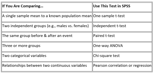
If this is still overwhelming consider getting SPSS help for students from an expert—or if you’re really stuck you might even think, Can I pay someone to do my statistics homework? (Spoiler: Yes, you can, but learning it yourself is worth it!)
3. Always Check for Normality – Don’t Skip This Step!
Most hypothesis tests assume your data is normally distributed. To check normality in SPSS:
Click Analyze > Descriptive Statistics > Explore
Move your dependent variable into the Dependent List box
Click Plots, check Normality Plots with Tests, then hit OK
Look at the Shapiro-Wilk test—if p > 0.05, your data is normal. If not, consider a non-parametric test like the Mann-Whitney U test instead of a t-test.
4. Understand the p-Value – It’s More Than Just < 0.05
A p-value tells you to reject H₀, but students often misinterpret it. If p < 0.05 you have significant results (reject H₀). If p > 0.05 the results are not statistically significant (fail to reject H₀).
But here’s the catch: A p-value alone doesn’t tell you if your results are practically significant. Always look at effect size and confidence intervals for more.
5. Check Assumptions Before You Run Any Test
Most tests require assumptions, like homogeneity of variance (for t-tests and ANOVA). In SPSS you can check this using Levene’s test:
Click Analyze > Compare Means > One-Way ANOVA
Check the box for Homogeneity of variance test
If p < 0.05, variances are unequal, and you may need to adjust (like Welch’s test).
Don’t skip assumption checks or you’ll end up with wrong conclusions!
6. Use Graphs to Back Up Your Hypothesis Testing
Raw numbers are great, but SPSS’s graphs will make your results more impressive. Try these:
Boxplots for comparing groups
Histograms to check distributions
Scatterplots to see correlations
To create graphs in SPSS go to Graphs > Legacy Dialogs, select your chart type and customize to make your results more obvious.
7. Know When to Use One-Tailed vs. Two-Tailed
Many students assume two-tailed tests are always the way to go. Not true!
One-tailed test if you have a specific directional hypothesis (e.g. "higher", "lower")
Two-tailed test if you’re just testing for any difference.
One-tailed tests are more powerful but you might miss the opposite effect. Choose wisely!
8. Is Your Sample Size Big Enough?
Small sample sizes can lead to wrong results. Use G*Power (free) or SPSS’s power analysis to check if your sample size is sufficient.
Click Analyze > Power Analysis
Enter your effect size, alpha level and expected sample size
If your study is underpowered (if so you may need more participants)
9. Write Up Your Results Like a Pro (APA Style)
If you’re writing a report follow APA style. Here’s how to write up your results:
"An independent t-test was conducted to compare test scores between students who used the app and those who didn’t. The results were significant, t(48) = 2.34, p = 0.022, d = 0.65, app users scored higher.”
Always include the test type, degrees of freedom, test statistic, p-value and effect size.
Final Thoughts
Hypothesis testing in SPSS doesn’t have to be torture. Follow these 9 tips—choose the right test, check assumptions, interpret results correctly—you’ll feel more confident and will ace your stats assignments. And remember, whenever you feel the need of SPSS help for students, don’t hesitate to reach out to your professor or online spss experts.
#SPSS help for students#spss#help in spss#Hypothesis Type#Statistical Test#Shapiro-Wilk test#Levene’s test#Power Analysis#G*Power#APA Style
0 notes
Text
Test a Basic Linear Reggression
Simple linear regression is used to estimate the relationship between two quantitative variables. You can use simple linear regression when you want to know:
How strong the relationship is between two variables (e.g., the relationship between rainfall and soil erosion).
The value of the dependent variable at a certain value of the independent variable (e.g., the amount of soil erosion at a certain level of rainfall).
Regression models describe the relationship between variables by fitting a line to the observed data. Linear regression models use a straight line, while logistic and nonlinear regression models use a curved line. Regression allows you to estimate how a dependent variable changes as the independent variable(s) change. Simple linear regression example .You are a social researcher interested in the relationship between income and happiness. You survey 500 people whose incomes range from 15k to 75k and ask them to rank their happiness on a scale from 1 to 10.
Your independent variable (income) and dependent variable (happiness) are both quantitative, so you can do a regression analysis to see if there is a linear relationship between them.
If you have more than one independent variable, use multiple linear regression instead.
Table of contents
Assumptions of simple linear regression
How to perform a simple linear regression
Interpreting the results
Presenting the results
Can you predict values outside the range of your data?
Other interesting articles
Frequently asked questions about simple linear regression
Assumptions of simple linear regression
Simple linear regression is a parametric test, meaning that it makes certain assumptions about the data. These assumptions are:
Homogeneity of variance (homoscedasticity): the size of the error in our prediction doesn’t change significantly across the values of the independent variable.
Independence of observations: the observations in the dataset were collected using statistically valid sampling methods, and there are no hidden relationships among observations.
Normality: The data follows a normal distribution.
Linear regression makes one additional assumption:
The relationship between the independent and dependent variable is linear: the line of best fit through the data points is a straight line (rather than a curve or some sort of grouping factor).
If your data do not meet the assumptions of homoscedasticity or normality, you may be able to use a nonparametric test instead, such as the Spearman rank test. Example: Data that doesn’t meet the assumptions.You think there is a linear relationship between cured meat consumption and the incidence of colorectal cancer in the U.S. However, you find that much more data has been collected at high rates of meat consumption than at low rates of meat consumption, with the result that there is much more variation in the estimate of cancer rates at the low range than at the high range. Because the data violate the assumption of homoscedasticity, it doesn’t work for regression, but you perform a Spearman rank test instead.
If your data violate the assumption of independence of observations (e.g., if observations are repeated over time), you may be able to perform a linear mixed-effects model that accounts for the additional structure in the data.
Prevent plagiarism. Run a free check.
How to perform a simple linear regression
Simple linear regression formula
The formula for a simple linear regression is:

y is the predicted value of the dependent variable (y) for any given value of the independent variable (x).
B0 is the intercept, the predicted value of y when the x is 0.
B1 is the regression coefficient – how much we expect y to change as x increases.
x is the independent variable ( the variable we expect is influencing y).
e is the error of the estimate, or how much variation there is in our estimate of the regression coefficient.
Linear regression finds the line of best fit line through your data by searching for the regression coefficient (B1) that minimizes the total error (e) of the model.
While you can perform a linear regression by hand, this is a tedious process, so most people use statistical programs to help them quickly analyze the data.
Simple linear regression in R
R is a free, powerful, and widely-used statistical program. Download the dataset to try it yourself using our income and happiness example.
Load the income.data dataset into your R environment, and then run the following command to generate a linear model describing the relationship between income and happiness: R code for simple linear regressionincome.happiness.lm <- lm(happiness ~ income, data = income.data)
This code takes the data you have collected data = income.data and calculates the effect that the independent variable income has on the dependent variable happiness using the equation for the linear model: lm().
To learn more, follow our full step-by-step guide to linear regression in R.
Interpreting the results
To view the results of the model, you can use the summary() function in R:summary(income.happiness.lm)
This function takes the most important parameters from the linear model and puts them into a table, which looks like this:

This output table first repeats the formula that was used to generate the results (‘Call’), then summarizes the model residuals (‘Residuals’), which give an idea of how well the model fits the real data.
Next is the ‘Coefficients’ table. The first row gives the estimates of the y-intercept, and the second row gives the regression coefficient of the model.
Row 1 of the table is labeled (Intercept). This is the y-intercept of the regression equation, with a value of 0.20. You can plug this into your regression equation if you want to predict happiness values across the range of income that you have observed:happiness = 0.20 + 0.71*income ± 0.018
The next row in the ‘Coefficients’ table is income. This is the row that describes the estimated effect of income on reported happiness:
The Estimate column is the estimated effect, also called the regression coefficient or r2 value. The number in the table (0.713) tells us that for every one unit increase in income (where one unit of income = 10,000) there is a corresponding 0.71-unit increase in reported happiness (where happiness is a scale of 1 to 10).
The Std. Error column displays the standard error of the estimate. This number shows how much variation there is in our estimate of the relationship between income and happiness.
The t value column displays the test statistic. Unless you specify otherwise, the test statistic used in linear regression is the t value from a two-sided t test. The larger the test statistic, the less likely it is that our results occurred by chance.
The Pr(>| t |) column shows the p value. This number tells us how likely we are to see the estimated effect of income on happiness if the null hypothesis of no effect were true.
Because the p value is so low (p < 0.001), we can reject the null hypothesis and conclude that income has a statistically significant effect on happiness.
The last three lines of the model summary are statistics about the model as a whole. The most important thing to notice here is the p value of the model. Here it is significant (p < 0.001), which means that this model is a good fit for the observed data.
Presenting the results
When reporting your results, include the estimated effect (i.e. the regression coefficient), standard error of the estimate, and the p value. You should also interpret your numbers to make it clear to your readers what your regression coefficient means: We found a significant relationship (p < 0.001) between income and happiness (R2 = 0.71 ± 0.018), with a 0.71-unit increase in reported happiness for every 10,000 increase in income.
It can also be helpful to include a graph with your results. For a simple linear regression, you can simply plot the observations on the x and y axis and then include the regression line and regression function:

Here's why students love Scribbr's proofreading services
Can you predict values outside the range of your data?
No! We often say that regression models can be used to predict the value of the dependent variable at certain values of the independent variable. However, this is only true for the range of values where we have actually measured the response.
We can use our income and happiness regression analysis as an example. Between 15,000 and 75,000, we found an r2 of 0.73 ± 0.0193. But what if we did a second survey of people making between 75,000 and 150,000?

The r2 for the relationship between income and happiness is now 0.21, or a 0.21-unit increase in reported happiness for every 10,000 increase in income. While the relationship is still statistically significant (p<0.001), the slope is much smaller than before.

What if we hadn’t measured this group, and instead extrapolated the line from the 15–75k incomes to the 70–150k incomes?
You can see that if we simply extrapolated from the 15–75k income data, we would overestimate the happiness of people in the 75–150k income range.

If we instead fit a curve to the data, it seems to fit the actual pattern much better.
It looks as though happiness actually levels off at higher incomes, so we can’t use the same regression line we calculated from our lower-income data to predict happiness at higher levels of income.
Even when you see a strong pattern in your data, you can’t know for certain whether that pattern continues beyond the range of values you have actually measured. Therefore, it’s important to avoid extrapolating beyond what the data actually tell you.
0 notes
Text
Data Analysis Using ANOVA Test with a Mediator
Blog Title: Data Analysis Using ANOVA Test with a Mediator
In this post, we will demonstrate how to test a hypothesis using the ANOVA (Analysis of Variance) test with a mediator. We will explain how ANOVA can be used to check for significant differences between groups, while focusing on how to include a mediator to understand the relationship between variables.
Hypothesis:
In this analysis, we assume that there is a significant effect of independent variables on the dependent variable, and we may test whether complex variables (such as the mediator) affect this relationship. In this context, we will test whether there are differences in health levels based on treatment types, while also checking how the mediator (stress level) influences this test.
1. Research Data:
Independent variable (X): Type of treatment (medication, physical therapy, or no treatment).
Dependent variable (Y): Health level.
Mediator (M): Stress level.
We will use the ANOVA test to determine whether there are differences in health levels based on treatment type and will assess how the mediator (stress level) influences this analysis.
2. Formula for ANOVA Test with a Mediator (Mediating Effect):
The formula we use for analyzing the data in ANOVA is as follows:Y=β0+β1X+β2M+β3(X×M)+ϵY = \beta_0 + \beta_1 X + \beta_2 M + \beta_3 (X \times M) + \epsilonY=β0+β1X+β2M+β3(X×M)+ϵ
Where:
YYY is the dependent variable (health level).
XXX is the independent variable (type of treatment).
MMM is the mediator variable (stress level).
β0\beta_0β0 is the intercept.
β1,β2,β3\beta_1, \beta_2, \beta_3β1,β2,β3 are the regression coefficients.
ϵ\epsilonϵ is the error term.
3. Analytical Steps:
A. Step One - ANOVA Analysis:
Initially, we apply the ANOVA test to the independent variable XXX (type of treatment) to determine if there are significant differences in health levels across different groups.
B. Step Two - Adding the Mediator:
Next, we add the mediator MMM (stress level) to our model to evaluate how stress could impact the relationship between treatment type and health level. This part of the analysis determines whether stress acts as a mediator affecting the treatment-health relationship.
4. Results and Output:
Let's assume we obtain ANOVA results with the mediator. The output might look like the following:
F-value for the independent variable XXX: Indicates whether there are significant differences between the groups.
p-value for XXX: Shows whether the differences between the groups are statistically significant.
p-value for the mediator MMM: Indicates whether the mediator has a significant effect.
p-value for the interaction between XXX and MMM: Reveals whether the interaction between treatment and stress significantly impacts the dependent variable.
5. Interpreting the Results:
After obtaining the results, we can interpret the following:
If the p-value for the variable XXX is less than 0.05, it means there is a statistically significant difference between the groups based on treatment type.
If the p-value for the mediator MMM is less than 0.05, it indicates that stress has a significant effect on health levels.
If the p-value for the interaction between XXX and MMM is less than 0.05, it suggests that the effect of treatment may differ depending on the level of stress.
6. Conclusion:
By using the ANOVA test with a mediator, we are able to better understand the relationship between variables. In this example, we tested how stress level can influence the relationship between treatment type and health. This kind of analysis provides deeper insights that can help inform health-related decisions based on strong data.
Example of Output from Statistical Software:
Formula Used in Statistical Software:
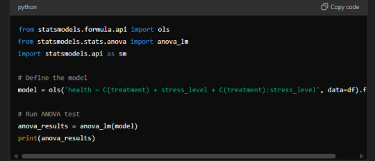
Sample Output:

Interpretation:
C(treatment): There are statistically significant differences between the groups in terms of treatment type (p-value = 0.0034).
stress_level: Stress has a significant effect on health (p-value = 0.0125).
C(treatment):stress_level: The interaction between treatment type and stress level shows a significant effect (p-value = 0.0435).
In summary, the results suggest that both treatment type and stress level have significant effects on health, and there is an interaction between the two that impacts health outcomes.
0 notes
Text
The Role of Statistics and Macroeconomics
A sound understanding of statistics and macroeconomics is highly important for students who are appearing for the entrance examination of the MA in Economics. Statistics forms a backbone for the interpretation of data in economics, and it enables students to analyze, interpret, and make informed predictions. The contrast between micro and macro involves the fact that macroeconomics gives the overall view of what happens in whole economies while discussing issues such as national income, inflation, and the government's policies. Together, these subjects make up the heart of economic analysis and are fundamental to pass the entrance exam.
Some Basic Concepts in Statistics in Economics
Statistics is at the heart of economics, where theories can be put to test, data can be interpreted, and meaningful conclusions can be drawn. Some of the main concepts in statistics to consider include the following:
Probability and Probability Distributions
Probability is the measure of uncertainty, often inherent in economic situations. A knowledge of the normal, binomial, and Poisson distributions is important for interpreting many economic occurrences and results.
Descriptive Statistics
Descriptive statistics is summarizing the data on one or more numerical measures of central tendency such as mean, median, mode along with measures of variation such as variance and standard deviation. These measures are used in order to identify patterns along with ascertaining central tendencies and variability of the datasets which shall enable economists to make preliminary observations.
Correlation and Regression Analysis
Correlation analysis provides information about the relationship between variables, but regression analysis extends that information to provide measures of the strength of the relationship between a dependent variable and one or more independent variables. The use of regression models is quite common in economics for understanding relationships among economic indicators, for instance, between income and consumption.
Hypothesis Testing
Hypothesis Testing. Hypothesis testing is a statistical methodology that gives the answer for whether an assumption about a population parameter is correct or not. It can be used to test a theory that might come from economics-a good example is investigating an effect of a policy change on inflation or unemployment.
Time Series Analysis
It is applied to analyze the economic data recorded with time, such as the growth rates of GDP, stock prices, and interest rates. With the use of moving averages and autoregressive models, one can estimate the future trends considering the existing data, which constitutes time series techniques.
Sampling and Estimation
Sampling techniques refer to the methods used to draw inferences about a larger population by conducting a sample survey. Estimation refers to making projections or generalizations regarding a population using sample data. The concepts covered include both point estimation and interval estimation. Mastering these statistical concepts will allow students to analyze and interpret economic data, becoming important in the exam and future economic studies.
Why is it crucial to understand Macroeconomics for the Exam?
Macroeconomics is also a core subject in the MA Economics syllabus that deals with the environment at large where some fundamental topic such as national income, inflation, unemployment, and economic policies is dealt with. Here are some key areas within macroeconomics especially relevant to the entrance exam:
National Income Accounting
National income accounting is the basis or framework on which the whole economic activity of the country is determined. Concepts such as Gross Domestic Product (GDP), Gross National Product (GNP), and Net National Product (NNP) explain the performance of a country's economy.
Aggregate Demand and Aggregate Supply
Aggregate demand is the total demand for goods and services; aggregate supply is the total supply of goods and services. These are two basic notions that explain most of the fluctuations in the economy and policy effects. Shifts in these curves explain inflation, recession, and other macroeconomic phenomena.
IS-LM Model
The IS-LM model is one of the most important tools in macroeconomics. It helps find out how the interest rate and the level of real output in goods and money markets are interlinked. Understanding the model will help the students predict what implications monetary and fiscal policies would make to the economy.
Inflation and Unemployment
The rate at which the price rises is called inflation while percentage of unemployed people is called unemployment. Both inflation and unemployment are among the most important indicators of economic health. Most of the times, concepts like the Phillips curve, which denotes the inverse relationship between inflation and unemployment, and theories about how control on inflation can be achieved, are tested.
Fiscal and Monetary Policies
Fiscal policy refers to the government spending and taxation policies while monetary policy is the central banks' power to influence money supply and interest rates. Since both these factors play an extremely influential role in stability within the economy, one needs to be familiar with these mechanisms in order to understand economic events and impacts of policies.
Growth Models of the Economy
It describes growth models, such as the Solow Growth Model, which will explain how factors contribute to long-run economic growth. They show what roles capital, labor, technology, and policy take in determining a country's economic development.
International Economics
Internationalization increased the importance of international economics which now constitutes an essential part of the macroeconomic study. Important ideas comprise a number of aspects, including exchange rates, trade policies, and balance of payments, between which economic systems interplay.
Knowledge of broad macroeconomic concepts enables the students to evaluate and understand large-scale economic behaviors besides outlining relationships between various economic variables.
How to Master These Subjects
Students need to study methodically if they are going to be able to become successful at statistics and macroeconomics. These are the dos and don'ts on how to master the subjects:
Major Concepts
Try to lay down a solid base of core concepts. In statistics, this will involve the following: probability, hypothesis testing, and regression analysis. For macroeconomics, it will involve national income accounting, IS-LM model, and fiscal and monetary policies.
Praction with Real Life Examples
Economics is a practically based subject. Applying statistical methods on real world economic data to interpret macroeconomic indicators would take the students a little deeper.
Web-based tools available, using the World Bank, IMF, and others, can be used to access easily even rudimentary economic data to be practiced on.
Use Visual Aids
Graphs and charts also help both subjects. Reinforce the ability to plot data with illustrations of how to estimate distributions and interpret the results of regressions graphically. For macroeconomics illustrate diagrams related to the IS-LM model, aggregate demand/supply curves, etc. to strengthen memory and understanding.
Continual Revision and Practice Questions
Practice makes perfect. Try previous year's question papers and sample questions to get yourself accustomed with the pattern of the exam. Most entrance exams have time limits, so practicing in a timed manner helps to gain speed and accuracy.
Time Management and Study Techniques
Statistics and macroeconomics is quite a vast syllabus. Managing time and an effective study schedule are quite necessary. Here are some techniques to help you
Formulate a Study Schedule
Plan out how you are going to spend your study time for each subject and be consistent in that. Spend more time on tough topics; also, you should be able to go over familiar concepts quite often.
Flashcards on Key Terms
Flashcards are really good for memorizing important terms and key concepts for the subjects. Especially with statistics, formulas have to be memorized; with macroeconomics, this is good practice in remembering the indicators and what they mean.
Group Study
Difficult subjects can be discussed with the help of group study. Fog can be removed through getting the insight of different people.
Take Regular Breaks
You may easily exhaust yourself if you sit down and just keep studying. You can get up, take breaks, refresh your mind, and stay focused and productive.
Keep Track of Your Progress
You must keep a journal to track your progress in all your subjects. This will enable you to realize where you need further improvement or in which areas you have done reasonably well.
Conclusion
Both statistics and macroeconomics have to be well mastered in order to ace the entrance examination to MA Economics. While statistics entails tools in handling data and testing hypotheses, macroeconomics equips you with understanding the overall economic environment and the relevant impacts of policy. Balancing your preparations between these subjects with special attention to core concepts and a highly efficient study schedule will maximize your prospects of getting through. With proper practice, use of strategic study techniques, and attention on how to apply this knowledge to reality, you will be better prepared to face the challenges associated with the MA Economics entrance exam.
0 notes
Text
Good questions!
I didn't expect this to take off the way it did. So when I was writing I was mostly just thinking of "being a petty asshole in front of my mutuals" and didn't really do my best to explain things well, but I'll try and answer the questions.
(also i make no claims of being better at statistics than the people who wrote this article. I hate stats and especially t-tests)
n=32: N is the sample size. The study had 32 ADHD subjects (and 28 neurotypicals). The larger the sample size, generally the lower the variance in the results: if you survey 1000 people you'll have a better idea than if you only survey 10.
44.4 ± 9.0 cm (1 sigma) is a way of specifying the mean and standard deviation of the sample. Focus on the first part: 44.4 cm. That means that for ADHD people, the average distance the center of gravity moved was 44.4 cm (in 25 seconds)
± 9.0 cm (1 sigma) The standard deviation is a measure of how spread-out the data is. The larger it is, the wider the spread. I don't have a great way to explain conceptually w/o diving into the math, so instead here's a possible distribution that matches those quoted means and standard deviations.

Hopefully that demonstrates that like, the ADHD distribution is maybe a little higher than the NT group if you squint at it, but not in a clean way?
P-values are a whole thing. They're the "chance that you'd get results like this if there was actually no correlation whatsoever". It's not a particularly intuitive number to understand. But like you said--p<0.05 is generally considered the bare minimum for scientific publication, and even that is not really sufficient in many cases.
(As an example of p values being a thing, they claim a significance of p=0.02, because they tested everybody 4 times, with eyes closed and open and stuff, and use that to 4x the sample size--it is my decidedly non-expert opinion that this is Bullshit, it'd be like if you asked me to shoot free throws 100 times, i only get 1 in, and you conclude from this that only 1% of tumblr users can make a free throw)
Some final thoughts:
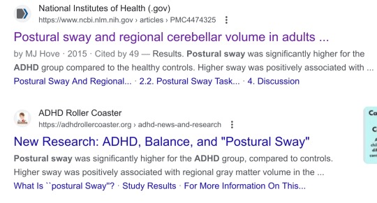
To be fair to the paper, there are some other papers on connection between ADHD and postural sway or other balance deficits. Here's a meta-analysis in children. To quote the abstract: "More than half of the children with ADHD have difficulties with gross and fine motor skills... The proportion of children with ADHD who improved their motor skills to the normal range by using medication varied from 28% to 67% between studies"
There does not seem to be any consensus on how or if the cerebellum is involved at all, or to what degree these balance deficits can be explained by the attention deficit or the hyperactivity vs being their own unique thing.
This really doesn't have anything to do with the dodging motion in the video, which I don't think really shows anything of the sort
To be unfair to the paper and the meta-analysis, it's also worth remembering that entire chunks of research fail to replicate ALL the time in psychology, especially in the 2000-2015 era this meta-analysis uses, which is squarely in the middle of the replication crisis.
every once in a while i learn some wild new piece of information that explains years of behavior and reminds me that i will never truly understand everything about my ridiculous adhd brain
#sorry this post kinda got long#FUCK wrong blog. this is kaiasky#i am not pasting all this into a new post sorry
59K notes
·
View notes
Text
What are the mathematical prerequisites for data science?
The key prerequisites for mathematics in Data Science would involve statistics and linear algebra.
Some of the important mathematical concepts one will encounter are as follows:
Statistics
Probability Theory: Probability distributions should be known, particularly normal, binomial, and Poisson, with conditional probability and Bayes' theorem. These will come in handy while going through statistical models and machine learning algorithms.
Descriptive Statistics: Measures of central tendency, mean, median, and mode, and measures of dispersion—variance and standard deviation—are very important in summarizing and getting an insight into data.
Inferential Statistics: In this part, the student is supposed to be conversant with hypothesis testing and confidence intervals in order to make inferences from samples back to populations and also to appreciate the concept of statistical significance.
Regression Analysis: This forms the backbone of modeling variable relationships through linear and logistic regression models.
Linear Algebra
Vectors and Matrices: This comprises vector and matrix operations—in particular, addition, subtraction, multiplication, transposition, and inversion.
Linear Equations: One can't work on regression analysis and dimensionality reduction without solving many systems of linear equations.
Eigenvalues and Eigenvectors: It forms the base of principal component analysis and other dimensionality reduction techniques.
Other Math Concepts
Calculus: This is not very core, like statistics and linear algebra, but it comes in handy while discussing gradient descent, optimization algorithms, and probability density functions.
Discrete Mathematics: Combinatorics and graph theory may turn out to be useful while going through some machine learning algorithms or even data structures.
Note: While these are the core mathematical requirements, the extent of mathematical background required varies with the specific area of interest within data science. For example, deep machine learning techniques require a deeper understanding of calculus and optimization.
0 notes
Text
Descriptive vs Inferential Statistics: What Sets Them Apart?

Statistics is a critical field in data science and research, offering tools and methodologies for understanding data. Two primary branches of statistics are descriptive and inferential statistics, each serving unique purposes in data analysis. Understanding the differences between these two branches "descriptive vs inferential statistics" is essential for accurately interpreting and presenting data.
Descriptive Statistics: Summarizing Data
Descriptive statistics focuses on summarizing and describing the features of a dataset. This branch of statistics provides a way to present data in a manageable and informative manner, making it easier to understand and interpret.
Measures of Central Tendency: Descriptive statistics include measures like the mean (average), median (middle value), and mode (most frequent value), which provide insights into the central point around which data values cluster.
Measures of Dispersion: It also includes measures of variability or dispersion, such as the range, variance, and standard deviation. These metrics indicate the spread or dispersion of data points in a dataset, helping to understand the consistency or variability of the data.
Data Visualization: Descriptive statistics often utilize graphical representations like histograms, bar charts, pie charts, and box plots to visually summarize data. These visual tools can reveal patterns, trends, and distributions that might not be apparent from numerical summaries alone.
The primary goal of descriptive statistics is to provide a clear and concise summary of the data at hand. It does not, however, make predictions or infer conclusions beyond the dataset itself.
Inferential Statistics: Making Predictions and Generalizations
While descriptive statistics focus on summarizing data, inferential statistics go a step further by making predictions and generalizations about a population based on a sample of data. This branch of statistics is essential when it is impractical or impossible to collect data from an entire population.
Sampling and Estimation: Inferential statistics rely heavily on sampling techniques. A sample is a subset of a population, selected in a way that it represents the entire population. Estimation methods, such as point estimation and interval estimation, are used to infer population parameters (like the population mean or proportion) based on sample data.
Hypothesis Testing: This is a key component of inferential statistics. It involves making a claim or hypothesis about a population parameter and then using sample data to test the validity of that claim. Common tests include t-tests, chi-square tests, and ANOVA. The results of these tests help determine whether there is enough evidence to support or reject the hypothesis.
Confidence Intervals: Inferential statistics also involve calculating confidence intervals, which provide a range of values within which a population parameter is likely to lie. This range, along with a confidence level (usually 95% or 99%), indicates the degree of uncertainty associated with the estimate.
Regression Analysis and Correlation: These techniques are used to explore relationships between variables and make predictions. For example, regression analysis can help predict the value of a dependent variable based on one or more independent variables.
Key Differences and Applications
The primary difference between descriptive and inferential statistics lies in their objectives. Descriptive statistics aim to describe and summarize the data, providing a snapshot of the dataset's characteristics. Inferential statistics, on the other hand, aim to make inferences and predictions about a larger population based on a sample of data.
In practice, descriptive statistics are often used in the initial stages of data analysis to get a sense of the data's structure and key features. Inferential statistics come into play when researchers or analysts want to draw conclusions that extend beyond the immediate dataset, such as predicting trends, making decisions, or testing hypotheses.
In conclusion, both descriptive and inferential statistics are crucial for data analysis and statistical analysis, each serving distinct roles. Descriptive statistics provide the foundation by summarizing data, while inferential statistics allow for broader generalizations and predictions. Together, they offer a comprehensive toolkit for understanding and making decisions based on data.
0 notes
Text
Homework 2 Problem 1 (20pts). Fundamental Knowledge for Generalization Theory
When the random variables can have negative values, the Markov inequality may fail. Give an example. How will sample size and variance in uence concentration? Explain it using Chebyshev’s inequality. Suppose X1; X2; ; Xn are i.i.d sub-Gaussian random variables with bounded variance, then we can apply both Chebyshev’s inequality and Hoe ding’s inequality. Discuss which bound is tighter. Explain…
0 notes
Text
Nonparametric Hypothesis Testing in Longitudinal Biostatistics: Assignment Help Notes
Biostatistics plays an important role in medical science and healthcare especially through observational studies involving specific health issues and their prevalence, risk factors and outcomes over a period of time. These studies involve longitudinal data in evaluating patients’ response to certain treatments and analyzing how specific risks evolve within a population over time. Hypothesis testing is crucial in ascertaining whether the observed patterns in the longitudinal data are statistically significant or not.
Although conventional parametric methods are largely used but they are not appropriate to real world scenarios due to the underlying assumptions such as normality, linearity and homoscedasticity. On the other hand, the nonparametric hypothesis testing remains a viable option for use since it doesn’t impose rigid assumptions on data distribution, particularly when dealing with complicated longitudinal data sets. However, students tend to face difficulties in nonparametric hypothesis testing due to the involvement of complex mathematical and statistical concepts and they often get confused while selecting the appropriate method for a specific dataset.
Let’s discuss about nonparametric hypothesis testing in detail.
What is Nonparametric Hypothesis Testing?
Hypothesis testing is aimed at determining whether the findings that are obtained from a given sample can be generalized to the larger population. The traditional parametric techniques such as t-test or analysis of variance (ANOVA) assumes normal data distributions with specific parameters such as mean and variance defining the population.
On the other hand, nonparametric hypothesis testing procedures make no assumption about the data distribution. Instead, it relies on ranks, medians, or other distribution-free approaches. This makes nonparametric tests particularly advantageous where the data do not meet the assumptions of a parametric test for example skewed distributions, outliers, or a non-linear association.
Common examples of nonparametric tests include:
Mann-Whitney U Test: For comparing two independent samples.
Wilcoxon Signed-Rank Test: For comparing two related samples.
Kruskal-Wallis Test: For comparing more than two independent samples.
Friedman Test: For comparing more than two related samples.
In longitudinal biostatistics, the data collected are usually measured over time, which complicates things further. The dependencies between repeated measures at different time points can violate parametric test assumptions, making nonparametric methods a better choice for many studies.
The Importance of Longitudinal Data
Longitudinal data monitors same subjects over time and serves valuable information for examining change in health outcomes. For instance, one might monitor a sample of patients with diabetes to discover how their blood sugar levels changed following commencement of new medication. Such data differs from cross-sectional data that only captures one time point.
The main difficulty of longitudinal data is the need to account for the correlation between repeated measurements. Measurements from the same subjects are usually similar as compared to measurements from different subjects, they can be treated as independent in the case of parametric tests.
Nonparametric Tests for Longitudinal Data
There are a number of nonparametric tests used to handle longitudinal data.
1. The Friedman Test:
This represents a nonparametric substitute for repeated-measures ANOVA. This is applied when you have information from the same subjects measured at various time periods. The Friedman test assigns ranks to the data for each time point and then measures whether there is a significant difference in the ranks across those time points.
Example:
Just imagine a dataset wherein three unique diets are under evaluation, at three separate time points, for a single group of patients. You are able to apply the Friedman test in python to assess if there is a major difference in health outcomes between the diets across time.
from scipy.stats import friedmanchisquare
# Sample data: each row represents a different subject, and each column is a time point
data = [[68, 72, 70], [72, 78, 76], [60, 65, 63], [80, 85, 83]]
# Perform the Friedman test
stat, p_value = friedmanchisquare(data[0], data[1], data[2], data[3])
print(f"Friedman Test Statistic: {stat}, P-Value: {p_value}")
It will furnish the Friedman test statistic as well as a p-value that conveys whether the difference are statistically significant.
2. The Rank-Based Mixed Model (RMM):
The Friedman test is quite effective with simple repeated measures, but it becomes less useful as longitudinal structures become more complex (e.g., unequal time points, missing data). The advanced method known as the rank-based mixed model can handle more complex scenarios. The RMMs differ from the Friedman test in that they are a mix of nonparametric and mixed models, providing flexible handling of random effects and the correlation between repeated measures.
Unfortunately, RMMs involve a range of complexities that typically need statistical software such as R or SAS for computation. Yet, their flexibility regarding longitudinal data makes them important for sophisticated biostatistical analysis.
3. The Wilcoxon Signed-Rank Test for Paired Longitudinal Data:
This test is a nonparametric replacement for a paired t-test when comparing two time points and is particularly beneficial when data is not normally distributed.
Example:
Imagine you are reviewing patients' blood pressure statistics before and after a certain treatment. The Wilcoxon Signed-Rank test can help you evaluate if there’s an notable difference at the two time points. Utilizing python,
from scipy.stats import wilcoxon
# Sample data: blood pressure readings before and after treatment
before = [120, 125, 130, 115, 140]
after = [118, 122, 128, 113, 137]
# Perform the Wilcoxon Signed-Rank test
stat, p_value = wilcoxon(before, after)
print(f"Wilcoxon Test Statistic: {stat}, P-Value: {p_value}")
Advantages of Nonparametric Tests
Flexibility: The nonparametric tests are more flexible than their parametric alternatives because the assumptions of data distribution is not required. This makes them perfect for the study of real-world data, which seldom requires assumptions needed by parametric methods.
Robustness to Outliers: Nonparametric tests utilize ranks in place of original data values, thereby increasing their resistance to the effect of outliers. This is important in biostatistics, since outliers (extreme values) can skew the results of parametric tests.
Handling Small Sample Sizes: Nonparametric tests typically work better for small sample sizes, a condition often found in medical studies, particularly in early clinical trials and pilot studies.
Also Read: Real World Survival Analysis: Biostatistics Assignment Help For Practical Skills
Biostatistics Assignment Help to Overcome Challenges in Nonparametric Methods
In spite of the advantages, many students find nonparametric methods hard to understand. An important problem is that these approaches commonly do not provide the sort of intuitive interpretation that parametric methods deliver. A t-test produces a difference in means, whereas nonparametric tests yield results based on rank differences, which can prove to be harder to conceptualize.
In addition, choosing between a nonparametric test and a parametric test can prove difficult, particularly when analyzing messy raw data. This decision regularly involves a profound grasp of the data as well as the underlying assumptions of numerous statistical tests. For beginners in the field, this may become too much to digest.
Availing biostatistics assignment help from an expert can prove to be a smart way to deal with these obstacles. Professionals can lead you through the details of hypothesis testing, inform you on selecting the right methods, and help you understand your results accurately.
Conclusion
Nonparametric hypothesis testing is a useful tool in longitudinal biostatistics for evaluating complex data that contradicts the assumptions of traditional parametric procedures. Understanding these strategies allows students to more successfully solve real-world research problems. However, because these methods are so complex, many students find it beneficial to seek professional biostatistics assignment help in order to overcome the complexities of the subject and ensure that they have a better comprehension of the subject matter and improve their problem-solving skills.
Users also ask these questions:
How do nonparametric tests differ from parametric tests in biostatistics?
When should I use a nonparametric test in a longitudinal study?
What are some common challenges in interpreting nonparametric test results?
Helpful Resources for Students
To expand your knowledge of nonparametric hypothesis testing in longitudinal biostatistics, consider the following resources:
"Biostatistical Analysis" by Jerrold H. Zar: This book offers a comprehensive introduction to both parametric and nonparametric methods, with examples relevant to biological research.
"Practical Nonparametric Statistics" by W.J. Conover: A detailed guide to nonparametric methods with practical applications.
"Applied Longitudinal Analysis" by Garrett M. Fitzmaurice et al.: This book focuses on the analysis of longitudinal data, including both parametric and nonparametric methods.
0 notes