#how to create random array in numpy python | Explore Tumblr Posts and Blogs

data-science-articles · 1 year

Text

How to Start Your Data Science Journey with Python: A Comprehensive Guide

Data science has emerged as a powerful field, revolutionizing industries with its ability to extract valuable insights from vast amounts of data. Python, with its simplicity, versatility, and extensive libraries, has become the go-to programming language for data science. Whether you are a beginner or an experienced programmer, this article will provide you with a comprehensive guide on how to start your data science journey with Python.

Understand the Fundamentals of Data Science:

Before diving into Python, it's crucial to grasp the fundamental concepts of data science. Familiarize yourself with key concepts such as data cleaning, data visualization, statistical analysis, and machine learning algorithms. This knowledge will lay a strong foundation for your Python-based data science endeavors.

Learn Python Basics:

Python is known for its readability and ease of use. Start by learning the basics of Python, such as data types, variables, loops, conditionals, functions, and file handling. Numerous online resources, tutorials, and interactive platforms like Codecademy, DataCamp, and Coursera offer comprehensive Python courses for beginners.

Master Python Libraries for Data Science:

Python's real power lies in its extensive libraries that cater specifically to data science tasks. Familiarize yourself with the following key libraries:

a. NumPy: NumPy provides powerful numerical computations, including arrays, linear algebra, Fourier transforms, and more.

b. Pandas: Pandas offers efficient data manipulation and analysis tools, allowing you to handle data frames effortlessly.

c. Matplotlib and Seaborn: These libraries provide rich visualization capabilities for creating insightful charts, graphs, and plots.

d. Scikit-learn: Scikit-learn is a widely-used machine learning library that offers a range of algorithms for classification, regression, clustering, and more.

Explore Data Visualization:

Data visualization plays a vital role in data science. Python libraries such as Matplotlib, Seaborn, and Plotly provide intuitive and powerful tools for creating visualizations. Practice creating various types of charts and graphs to effectively communicate your findings.

Dive into Data Manipulation with Pandas:

Pandas is an essential library for data manipulation tasks. Learn how to load, clean, transform, and filter data using Pandas. Master concepts like data indexing, merging, grouping, and pivoting to manipulate and shape your data effectively.

Gain Statistical Analysis Skills:

Statistical analysis is a core aspect of data science. Python's Scipy library offers a wide range of statistical functions, hypothesis testing, and probability distributions. Acquire the knowledge to analyze data, draw meaningful conclusions, and make data-driven decisions.

Implement Machine Learning Algorithms:

Machine learning is a key component of data science. Scikit-learn provides an extensive range of machine learning algorithms. Start with simpler algorithms like linear regression and gradually progress to more complex ones like decision trees, random forests, and support vector machines. Understand how to train models, evaluate their performance, and fine-tune them for optimal results.

Explore Deep Learning with TensorFlow and Keras:

For more advanced applications, delve into deep learning using Python libraries like TensorFlow and Keras. These libraries offer powerful tools for building and training deep neural networks. Learn how to construct neural network architectures, handle complex data types, and optimize deep learning models.

Participate in Data Science Projects:

To solidify your skills and gain practical experience, engage in data science projects. Participate in Kaggle competitions or undertake personal projects that involve real-world datasets. This hands-on experience will enhance your problem-solving abilities and help you apply your knowledge effectively.

Continuously Learn and Stay Updated:

The field of data science is constantly evolving, with new techniques, algorithms, and libraries emerging.

Conclusion:

Embarking on your data science journey with Python opens up a world of opportunities to extract valuable insights from data. By following the steps outlined in this comprehensive guide, you can lay a solid foundation and start your data science endeavors with confidence.

Python's versatility and the abundance of data science libraries, such as NumPy, Pandas, Matplotlib, Scikit-learn, TensorFlow, and Keras, provide you with the necessary tools to manipulate, analyze, visualize, and model data effectively. Remember to grasp the fundamental concepts of data science, continuously learn and stay updated with the latest advancements in the field.

Engaging in data science projects and participating in competitions will further sharpen your skills and enable you to apply your knowledge to real-world scenarios. Embrace challenges, explore diverse datasets, and seek opportunities to collaborate with other data scientists to expand your expertise and gain valuable experience.

Data science is a journey that requires perseverance, curiosity, and a passion for solving complex problems. Python, with its simplicity and powerful libraries, provides an excellent platform to embark on this journey. So, start today, learn Python, and unlock the boundless potential of data science to make meaningful contributions in your field of interest.

#python #datascience #career #education #skillslash #student #courses #coding

0 notes

tutorialwithexample · 1 year

Text

Python NumPy Tutorial: A Comprehensive Guide for Scientific Computing

Python NumPy is a popular library for scientific computing that enables users to perform complex mathematical operations quickly and efficiently. In this Python NumPy tutorial, we will cover everything you need to know to get started with Python NumPy.

First, we will cover the installation process and how to create NumPy arrays. Next, we will dive into array manipulation techniques such as indexing, slicing, and reshaping. We will also cover mathematical operations such as addition, subtraction, and multiplication.

For more advanced users, we will cover topics such as broadcasting, masking, and random sampling. We will provide real-world examples and code snippets to help you understand the concepts.

#Python NumPy Tutorial

0 notes

mypythonteacher · 2 years

Text

NumPy

The crown jewel of NumPy is the ndarray. The ndarray is a homogeneous n-dimensional array object. What does that mean? 🤨

A Python List or a Pandas DataFrame can contain a mix of strings, numbers, or objects (i.e., a mix of different types). Homogenous means all the data have to have the same data type, for example all floating-point numbers.

And n-dimensional means that we can work with everything from a single column (1-dimensional) to the matrix (2-dimensional) to a bunch of matrices stacked on top of each other (n-dimensional).

To import NumPy: import numpy as np

To make a 1-D Array (Vector): my_array = np.array([1.1, 9.2, 8.1, 4.7])

To get the shape (rows, columns): my_array.shape

To access a particular value by the index: my_array[2]

To get how many dimensions there are: my_array.ndim

To make a 2D Array (matrix):

array_2d = np.array([[1, 2, 3, 9],

[5, 6, 7, 8]])

To get the shape (columns, rows): array_2d.shape

To get a particular 1D vector: mystery_array[2, 1, :]

Use .arange()to createa a vector a with values ranging from 10 to 29: a = np.arange(10, 30)

The last 3 values in the array: a[-3:]

An interval between two values: a[3:6]

All the values except the first 12: a[12:]

Every second value; a[::2]

To reverse an array: f = np.flip(a) OR a[::-1]

To get the indices of the non-zero elements in an array: nz_indices = np.nonzero(b)

To generate a random 3x3x3 array:

from numpy.random import random

z = random((3,3,3))

or use the full path to call it.

z = np.random.random((3,3,3)) # without an import statement

print(z.shape)

random_array = np.random.rand(3, 3, 3)

print(random_array)

To create a vector of size 9 from 0 to 100 with values evenly spaced: x = np.linspace(0,100, num=9)

To create an array called noise and display it as an image:

noise = np.random.random((128,128,3))

print(noise.shape)

plt.imshow(noise)

To display a random picture of a raccoon:

img = misc.face()

plt.imshow(img)

0 notes

karanshah1910 · 4 years

Text

Master NumPy Library for Data Analysis in Python in 10 Minutes

Learn and Become a Master of one of the most used Python tools for Data Analysis.

Introduction:-

NumPy is a python library used for working with arrays.It also has functions for working in domain of linear algebra, fourier transform, and matrices.It is an open source project and you can use it freely. NumPy stands for Numerical Python.

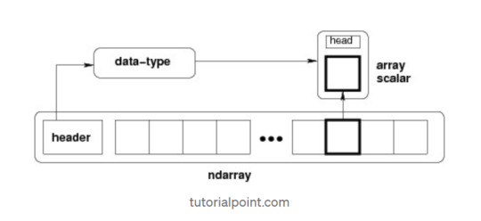
NumPy — Ndarray Object

The most important object defined in NumPy is an N-dimensional array type called ndarray. It describes the collection of items of the same type. Items in the collection can be accessed using a zero-based index.Every item in an ndarray takes the same size of block in the memory.

Each element in ndarray is an object of data-type object (called dtype).Any item extracted from ndarray object (by slicing) is represented by a Python object of one of array scalar types.

The following diagram shows a relationship between ndarray, data type object (dtype) and array scalar type −

It creates an ndarray from any object exposing array interface, or from any method that returns an array.

numpy.array(object, dtype = None, copy = True, order = None, subok = False, ndmin = 0)

The above constructor takes the following parameters −

Object :- Any object exposing the array interface method returns an array, or any (nested) sequence.

Dtype : — Desired data type of array, optional.

Copy :- Optional. By default (true), the object is copied.

Order :- C (row major) or F (column major) or A (any) (default).

Subok :- By default, returned array forced to be a base class array. If true, sub-classes passed through.

ndmin :- Specifies minimum dimensions of resultant array.

Operations on Numpy Array

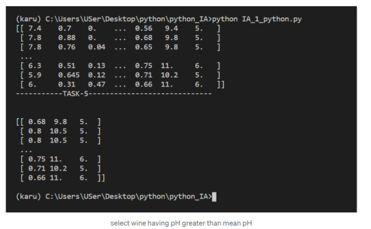
In this blog, we’ll walk through using NumPy to analyze data on wine quality. The data contains information on various attributes of wines, such as pH and fixed acidity, along with a quality score between 0 and 10 for each wine. The quality score is the average of at least 3 human taste testers. As we learn how to work with NumPy, we’ll try to figure out more about the perceived quality of wine.

The data was downloaded from the winequality-red.csv, and is available here. file, which we’ll be using throughout this tutorial:

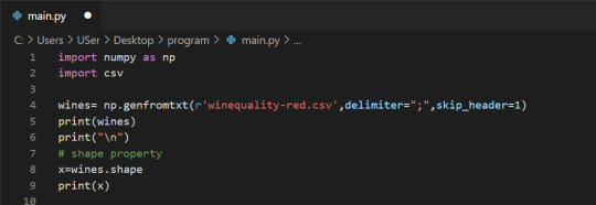
Lists Of Lists for CSV Data

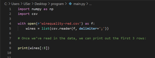
Before using NumPy, we’ll first try to work with the data using Python and the csv package. We can read in the file using the csv.reader object, which will allow us to read in and split up all the content from the ssv file.

In the below code, we:

Import the csv library.

Open the winequality-red.csv file.

With the file open, create a new csv.reader object.

Pass in the keyword argument delimiter=";" to make sure that the records are split up on the semicolon character instead of the default comma character.

Call the list type to get all the rows from the file.

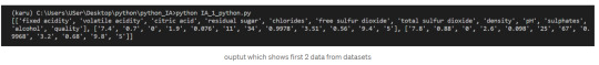
Assign the result to wines.

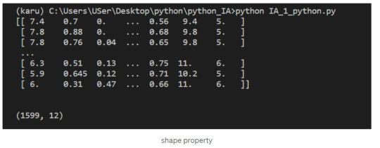
We can check the number of rows and columns in our data using the shape property of NumPy arrays:

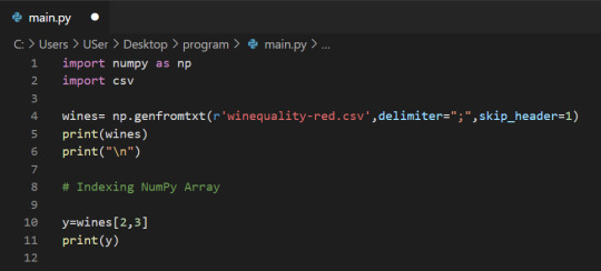
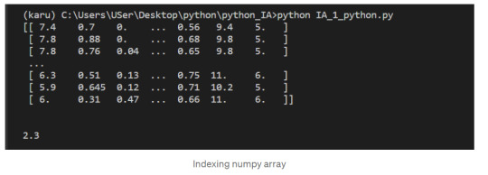
Indexing NumPy Arrays

Let’s select the element at row 3 and column 4. In the below code, we pass in the index 2 as the row index, and the index 3 as the column index. This retrieves the value from the fourth column of the third row:

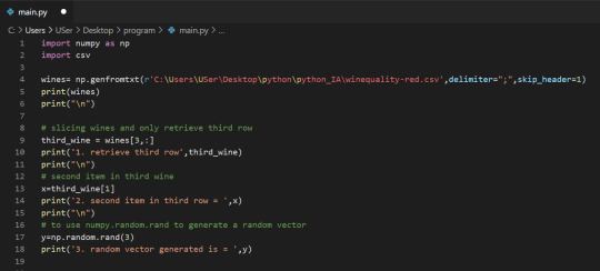
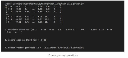
1-Dimensional NumPy Arrays

So far, we’ve worked with 2-dimensional arrays, such as wines. However, NumPy is a package for working with multidimensional arrays. One of the most common types of multidimensional arrays is the 1-dimensional array, or vector.

1.Just like a list of lists is analogous to a 2-dimensional array, a single list is analogous to a 1-dimensional array. If we slice wines and only retrieve the third row, we get a 1-dimensional array:

2. We can retrieve individual elements from third_wine using a single index. The below code will display the second item in third_wine:

3. Most NumPy functions that we’ve worked with, such as numpy.random.rand, can be used with multidimensional arrays. Here’s how we’d use numpy.random.rand to generate a random vector:

After successfully reading our dataset and learning about List, Indexing, & 1D array in NumPy we can start performing the operation on it.

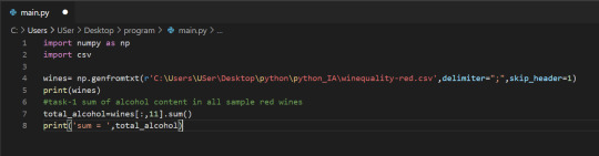
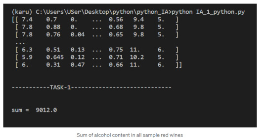
The first element of each row is the fixed acidity, the second is the volatile ,acidity, and so on. We can find the average quality of the wines. The below code will:

Extract the last element from each row after the header row.

Convert each extracted element to a float.

Assign all the extracted elements to the list qualities.

Divide the sum of all the elements in qualities by the total number of elements in qualities to the get the mean.

NumPy Array Methods

In addition to the common mathematical operations, NumPy also has several methods that you can use for more complex calculations on arrays. An example of this is the numpy.ndarray.sum method. This finds the sum of all the elements in an array by default:

2. Sum of alcohol content in all sample red wines

NumPy Array Comparisons

We get a Boolean array that tells us which of the wines have a quality rating greater than 5. We can do something similar with the other operators. For instance, we can see if any wines have a quality rating equal to 10:

3. select wines having pH content > 5

Subsetting

We select only the rows where high_Quality contains a True value, and all of the columns. This subsetting makes it simple to filter arrays for certain criteria. For example, we can look for wines with a lot of alcohol and high quality. In order to specify multiple conditions, we have to place each condition in parentheses, and separate conditions with an ampersand (&):

4. Select only wines where sulphates >10 and alcohol >7

5. select wine having pH greater than mean pH

We have seen what NumPy is, and some of its most basic uses. In the following posts we will see more complex functionalities and dig deeper into the workings of this fantastic library!

To check it out follow me on tumblr, and stay tuned!

That is all, I hope you liked the post. Feel Free to follow me on tumblr

Also, you can take a look at my other posts on Data Science and Machine Learning here. Have a good read!

#data science #machine learning #data analysis #python #numpy #data extraction

1 note · View note

sbrocks99 · 4 years

Text

Running a Random Forest

Hey guy’s welcome back in previous blog we have seen that, how to run classification trees in python you can check it here. In this blog you are going to learn how to run Random Forest using python.

So now let's see how to generate a random forest with Python. Again, I'm going to use the Wave One, Add Health Survey that I have data managed for the purpose of growing decision trees. You'll recall that there are several variables. Again, we'll define the response or target variable, regular smoking, based on answers to the question, have you ever smoked cigarettes regularly? That is, at least one cigarette every day for 30 days.

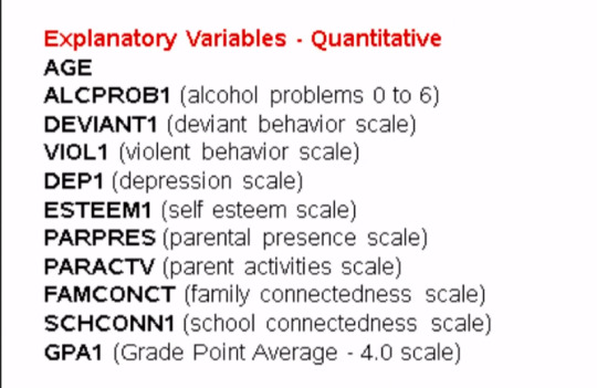
The candidate explanatory variables include gender, race, alcohol, marijuana, cocaine, or inhalant use. Availability of cigarettes in the home, whether or not either parent was on public assistance, any experience with being expelled from school, age, alcohol problems, deviance, violence, depression, self esteem, parental presence, activities with parents family and school connectedness and grade point average.

Much of the code that we'll write for our random forest will be quite similar to the code we had written for individual decision trees.

First there are a number of libraries that we need to call in, including features from the sklearn library.

from pandas import Series, DataFrame import pandas as pd import numpy as np import os import matplotlib.pylab as plt from sklearn.cross_validation import train_test_split from sklearn.tree import DecisionTreeClassifier from sklearn.metrics import classification_report import sklearn.metrics # Feature Importance from sklearn import datasets from sklearn.ensemble import ExtraTreesClassifier

Next I'm going to use the change working directory function from the OS library to indicate where my data set is located.

os.chdir("C:\TREES")

Next I'll load my data set called tree_addhealth.csv. because decision tree analyses cannot handle any NAs in our data set, my next step is to create a clean data frame that drops all NAs. Setting the new data frame called data_clean I can now take a look at various characteristics of my data, by using the D types and describe functions to examine data types and summary statistics.

#Load the dataset

AH_data = pd.read_csv("tree_addhealth.csv") data_clean = AH_data.dropna()

data_clean.dtypes data_clean.describe()

Next I set my explanatory and response, or target variables, and then include the train test split function for predictors and target. And set the size ratio to 60% for the training sample, and 40% for the test sample by indicating test_size=.4.

#Split into training and testing sets

predictors = data_clean[['BIO_SEX','HISPANIC','WHITE','BLACK','NAMERICAN','ASIAN','age', 'ALCEVR1','ALCPROBS1','marever1','cocever1','inhever1','cigavail','DEP1','ESTEEM1','VIOL1', 'PASSIST','DEVIANT1','SCHCONN1','GPA1','EXPEL1','FAMCONCT','PARACTV','PARPRES']]

targets = data_clean.TREG1

Here I request the shape of these predictor and target and training test samples.

pred_train.shape pred_test.shape tar_train.shape tar_test.shape

From sklearn.ensamble I import the RandomForestClassifier

#Build model on training data from sklearn.ensemble import RandomForestClassifier

Now that training and test data sets have already been created, we'll initialize the random forest classifier from SK Learn and indicate n_estimators=25. n_estimators are the number of trees you would build with the random forest algorithm.

classifier=RandomForestClassifier(n_estimators=25)

Next I actually fit the model with the classifier.fit function which we passed the training predictors and training targets too.

classifier=classifier.fit(pred_train,tar_train)

Then, we go unto the prediction on the testator set. And we could also similar to decision tree code as for the confusion matrix and accuracy scores.

predictions=classifier.predict(pred_test)

sklearn.metrics.confusion_matrix(tar_test,predictions) sklearn.metrics.accuracy_score(tar_test, predictions)

For the confusion matrix, we see the true negatives and true positives on the diagonal. And the 207 and the 82 represent the false negatives and false positives, respectively. Notice that the overall accuracy for the forest is 0.84. So 84% of the individuals were classified correctly, as regular smokers, or not regular smokers.

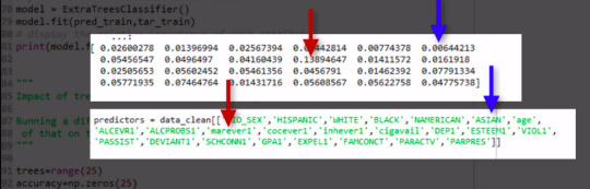
Given that we don't interpret individual trees in a random forest, the most helpful information to be gotten from a forest is arguably the measured importance for each explanatory variable. Also called the features. Based on how many votes or splits each has produced in the 25 tree ensemble. To generate importance scores, we initialize the extra tree classifier, and then fit a model. Finally, we ask Python to print the feature importance scores calculated from the forest of trees that we've grown.

# fit an Extra Trees model to the data model = ExtraTreesClassifier() model.fit(pred_train,tar_train) # display the relative importance of each attribute print(model.feature_importances_)

The variables are listed in the order they've been named earlier in the code. Starting with gender, called BIO_SEX, and ending with parental presence. As we can see the variables with the highest important score at 0.13 is marijuana use. And the variable with the lowest important score is Asian ethnicity at .006.

As you will recall, the correct classification rate for the random forest was 84%. So were 25 trees actually needed to get this correct rate of classification? To determine what growing larger number of trees has brought us in terms of correct classification. We're going to use code that builds for us different numbers of trees, from one to 25, and provides the correct classification rate for each. This code will build for us random forest classifier from one to 25, and then finding the accuracy score for each of those trees from one to 25, and storing it in an array. This will give me 25 different accuracy values. And we'll plot them as the number of trees increase.

""" Running a different number of trees and see the effect of that on the accuracy of the prediction """

trees=range(25) accuracy=np.zeros(25)

for idx in range(len(trees)): classifier=RandomForestClassifier(n_estimators=idx + 1) classifier=classifier.fit(pred_train,tar_train) predictions=classifier.predict(pred_test) accuracy[idx]=sklearn.metrics.accuracy_score(tar_test, predictions)

plt.cla() plt.plot(trees, accuracy)

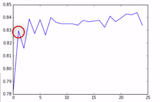
As you can see, with only one tree the accuracy is about 83%, and it climbs to only about 84% with successive trees that are grown giving us some confidence that it may be perfectly appropriate to interpret a single decision tree for this data. Given that it's accuracy is quite near that of successive trees in the forest.

To summarize, like decision trees, random forests are a type of data mining algorithm that can select from among a large number of variables. Those that are most important in determining the target or response variable to be explained.

Also light decision trees. The target variable in a random forest can be categorical or quantitative. And the group of explanatory variables or features can be categorical and quantitative in any combination. Unlike decision trees however, the results of random forests often generalize well to new data.

Since the strongest signals are able to emerge through the growing of many trees. Further, small changes in the data do not impact the results of a random forest. In my opinion, the main weakness of random forests is simply that the results are less satisfying, since no trees are actually interpreted. Instead, the forest of trees is used to rank the importance of variables in predicting the target.

Thus we get a sense of the most important predictive variables but not necessarily their relationships to one another.

Complete Code

os.chdir("C:\TREES")

#Load the dataset

AH_data = pd.read_csv("tree_addhealth.csv") data_clean = AH_data.dropna()

data_clean.dtypes data_clean.describe()

#Split into training and testing sets

targets = data_clean.TREG1

pred_train, pred_test, tar_train, tar_test = train_test_split(predictors, targets, test_size=.4)

pred_train.shape pred_test.shape tar_train.shape tar_test.shape

#Build model on training data from sklearn.ensemble import RandomForestClassifier

classifier=RandomForestClassifier(n_estimators=25) classifier=classifier.fit(pred_train,tar_train)

predictions=classifier.predict(pred_test)

sklearn.metrics.confusion_matrix(tar_test,predictions) sklearn.metrics.accuracy_score(tar_test, predictions)

# fit an Extra Trees model to the data model = ExtraTreesClassifier() model.fit(pred_train,tar_train) # display the relative importance of each attribute print(model.feature_importances_)

""" Running a different number of trees and see the effect of that on the accuracy of the prediction """

trees=range(25) accuracy=np.zeros(25)

plt.cla() plt.plot(trees, accuracy)

If you are still here, I appreciate that, and see you guy’s next time. ✌️

1 note · View note

gayatrisc · 4 years

Text

Top 8 Python Libraries for Data Science

Python language is popular and most commonly used by developers in creating mobile apps, games and other applications. A Python library is nothing but a collection of functions and methods which helps in solving complex data science-related functions. Python also helps in saving an amount of time while completing specific tasks.

Python has more than 130,000 libraries that are intended for different uses. Like python imaging library is used for image manipulation whereas Tensorflow is used for the development of Deep Learning models using python.

There are multiple python libraries available for data science and some of them are already popular, remaining are improving day-by-day to reach their acceptance level by developers

Read: HOW TO SHAPE YOUR CAREER WITH DATA SCIENCE COURSE IN BANGALORE?

Here we are discussing some Python libraries which are used for Data Science:

1. Numpy

NumPy is the most popular library among developers working on data science. It is used for performing scientific computations like a random number, linear algebra and Fourier transformation. It can also be used for binary operations and for creating images. If you are in the field of Machine Learning or Data Science, you must have good knowledge of NumPy to process your real-time data sets. It is a perfect tool for basic and advanced array operations.

2. Pandas

PANDAS is an open-source library developed over Numpy and it contains Data Frame as its main data structure. It is used in high-performance data structures and analysis tools. With Data Frame, we can manage and store data from tables by performing manipulation over rows and columns. Panda library makes it easier for a developer to work with relational data. Panda offers fast, expressive and flexible data structures.

Translating complex data operations using mere one or two commands is one of the most powerful features of pandas and it also features time-series functionality.

3. Matplotlib

This is a two-dimensional plotting library of Python a programming language that is very famous among data scientists. Matplotlib is capable of producing data visualizations such as plots, bar charts, scatterplots, and non-Cartesian coordinate graphs.

It is one of the important plotting libraries’ useful in data science projects. This is one of the important library because of which Python can compete with scientific tools like MatLab or Mathematica.

4. SciPy

SciPy library is based on the NumPy concept to solve complex mathematical problems. It comes with multiple modules for statistics, integration, linear algebra and optimization. This library also allows data scientist and engineers to deal with image processing, signal processing, Fourier transforms etc.

If you are going to start your career in the data science field, SciPy will be very helpful to guide you for the whole numerical computations thing.

5. Scikit Learn

Scikit-Learn is open-sourced and most rapidly developing Python libraries. It is used as a tool for data analysis and data mining. Mainly it is used by developers and data scientists for classification, regression and clustering, stock pricing, image recognition, model selection and pre-processing, drug response, customer segmentation and many more.

6. TensorFlow

It is a popular python framework used in deep learning and machine learning and it is developed by Google. It is an open-source math library for mathematical computations. Tensorflow allows python developers to install computations to multiple CPU or GPU in desktop, or server without rewriting the code. Some popular Google products like Google Voice Search and Google Photos are built using the Tensorflow library.

7. Keras

Keras is one of the most expressive and flexible python libraries for research. It is considered as one of the coolest machine learning Python libraries offer the easiest mechanism for expressing neural networks and having all portable models. Keras is written in python and it has the ability to run on top of Theano and TensorFlow.

Compared to other Python libraries, Keras is a bit slow, as it creates a computational graph using the backend structure and then performs operations.

8. Seaborn

It is a data visualization library for a python based on Matplotlib is also integrated with pandas data structures. Seaborn offers a high-level interface for drawing statistical graphs. In simple words, Seaborn is an extension of Matplotlib with advanced features.

Matplotlib is used for basic plotting such as bars, pies, lines, scatter plots and Seaborn is used for a variety of visualization patterns with few syntaxes and less complexity.

With the development of data science and machine learning, Python data science libraries are also advancing day by day. If you are interested in learning python libraries in-depth, get NearLearn’s Best Python Training in Bangalore with real-time projects and live case studies. Other than python, we provide training on Data Science, Machine learning, Blockchain and React JS course. Contact us to get to know about our upcoming training batches and fees.

Call: +91-80-41700110

Mail: [email protected]

#Top Python Training in Bangalore #Best Python Course in Bangalore #Best Python Course Training in Bangalore #Best Python Training Course in Bangalore #Python Course Fees in Bangalore

1 note · View note

marialaura-diazpena · 3 years

Text

My Programming Journey: Machine Learning using Python

After learning how to code in SAIT I decided I wanted to take things to the next level with my programming skills and try Machine Learning by myself, given that Artificial Intelligence has always been a really intriguing topic for me and I like a good old challenge to improve, grow and, most importantly, learn new things.

A lot is said about Machine Learning, but we can define it as algorithms that gather/analyze data and learn automatically through experience without being programmed to do so. The learning is done by identifying patterns and making decisions or predictions based on the data.

ML is not a new technology but recently has been growing rapidly and being used in everyday life. Examples that we are all familiar with are:

-Predictions in Search Engines

-Content recommendations from stream services or social media platforms

-Spam detection in emails

-Self-driving cars

-Virtual assistants

The Importance of Machine Learning

The vast amount of data available and processing power in modern technology makes it the perfect environment to train machine-learning models and by building precise models an organization can make better decisions. Most industries that deal with big data recognize the value of ML technology. In the health care industry, this technology has made it easier to diagnose patients, provide treatment plans and even perform precision surgeries. Government agencies and financial services also benefit from machine-learning since they deal with large amounts of data. This data is often used for insights and security, like preventing identity theft and fraud.

Other things like speech and language recognition, facial recognition for surveillance, transcription and translation of speech and computer vision are all thanks to machine learning, and the list goes on.

Types of Machine Learning

Usually, machine learning is divided into three categories: supervised learning, unsupervised learning and reinforcement learning.

Supervised learning

For this approach, machines are exposed to labelled data and learn by example. The algorithm receives a set of inputs with the correct outputs and learns by comparing its output with the correct output and modify the model as needed. The most common supervised learning algorithms are classification, regression and artificial neural networks.

Unsupervised learning

Unlike the previous approach, the unsupervised learning method takes unlabelled data so that the algorithm can identify patterns in data. Popular algorithms include nearest-neighbor mapping and k-means clustering.

Reinforcement learning

This approach consists of the algorithm interacting with the environment to find the actions that give the biggest rewards as feedback.

Iris Flower Classification Project

The iris flower problem is the “Hello World” of machine learning.

Iris flowers in Vancouver Park by Kevin Castel in Unsplash - https://unsplash.com/photos/y4xISRK8TUg

I felt tempted to try a machine learning project that I knew was too advanced for me and flex a little or fail miserably, but I decided to start with this iconic project instead. The project consists of classifying iris flowers among three species from measurements of sepals and petals’ length and width. The iris dataset contains 3 classes of 50 instances each, with classes referring to a type of iris flower.

Before Starting the Project

For this project, and for the rest of my machine learning journey, I decided to install Anaconda (Python 3.8 distribution), a package management service that comes with the best python libraries for data science and with many editors, including Visual Studio Code, the editor I will be using for this demonstration.

You can get Anaconda here: https://repo.anaconda.com/archive/Anaconda3-2021.05-Windows-x86_64.exe

I find that Anaconda makes it easy to access Python environments and it contains a lot of other programs to code and practice, as well as nice tutorials to get acquainted with the software.

In the following videos, I will be going step by step on the development of this project:

youtube

If videos aren't your thing, the readable step-by-step instructions are here in the post:

Prior to this project, I already had Visual Studio Code installed on my computer since I had used it for previous semesters. From VSCode I installed Python and then I selected a Python interpreter. The Python interpreter I will use is Anaconda, because it has all the dependencies I need for coding.

Getting Started

I configured Visual Studio Code to be able to develop in Python, then I created a python file named ml-iris.py and imported the libraries, which are the following:

The main libraries I will be using are numpyand sklearn.

· Numpy supports large, multidimensional arrays and a vast collection of mathematical operations to apply on these arrays.

· Sklearn includes various algorithms like classification, regression and clustering, the dataset used is embedded in sklearn.

From the previously mentioned libraries, I am using the following methods:

· load_iris is the data source of the Iris Flowers dataset

· train_test_split is the method to split the dataset

· KNeighborsClassifier is the method to classify the dataset.

I will be applying a supervised learning type of ML to this project: I already know the measurements of the three kinds of iris species; setosa, versicolor or virginica. From these measurements, I know which species each flower belongs to. So, what I want is to build a model that learns from the features of these already known irises and then predicts one of the species of iris when given new data, this means new irises flowers.

Now I start building the model:

The first step (line 6), I define the dataset by loading the load_iris() dataset from Sklearn.

Next step (line 7), I retrieve the target names information from the dataset, then format it and print it.

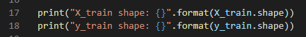
I repeat this step for retrieval of feature names, type and shape of data, type and shape of target, as well as target information (lines 8 to 13).

Target names should be Setosa, Versicolor and Virginica.

Feature names should be sepal length, sepal width, petal length and petal width.

Type of data should be a numpy array.

Shape of data is the shape of the array, which is 150 samples with 4 features each.

Type of target is a numpy array.

Shape of target is 150 samples.

The target is the list of all the samples, identified as numbers from 0 to 2.

· Setosa (0)

· Versicolor(1)

· Virginica(2)

Now I need to test the performance of my model, so I will show it new data, already labelled.

For this, I need to split the labelled data into two parts. One part will be used to train the model and the rest of the data will be used to test how the model works.

This is done by using the train_test_split function. The training set is x_train and y_train. The testing set is x_test and y_test. These sets are defined by calling the previously mentioned function (line 15). The arguments for the function are samples (data), features (target) and a random seed. This should return 4 datasets.

The function extracts ¾ of the labelled data as the training set and the remainder ¼ of the labelled data will be used as the test set.

Then I will print the shape of the training sets:

And the shape of the testing sets:

Now that the training and testing sets are defined, I can start building the model.

For this, I will use the K nearest neighbors classifier, from the Sklearn library.

This algorithm classifies a data point by its neighbors (line 23), with the data point being allocated to the class most common among its K nearest neighbors. The model can make a prediction by using the majority class among the neighbors. The k is a user-defined constant (I used 1), and a new data point is classified by assigning the label which is most frequent among the k training samples nearest to that data point.

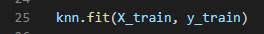
By using the fit method of the knn object (K Nearest Neighbor Classifier), I am building the model on the training set (line 25). This allows me to make predictions on any new data that comes unlabelled.

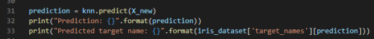
Here I create new data (line 27), sepal length(5), sepal width(2.9), petal length(1) and petal witdth(0.2) and put it into an array, calculate its shape and print it (line 28), which should be 1,4. The 1 being the number of samples and 4 being the number of features.

Then I call the predict method of the knn object on the new data:

The model predicts in which class this new data belongs, prints the prediction and the predicted target name (line 32, 32).

Now I have to measure the model to make sure that it works and I can trust its results. Using the testing set, my model can make a prediction for each iris it contains and I can compare it against its label. To do this I need the accuracy.

I use the predict method of the knn object on the testing dataset (line 36) and then I print the predictions of the test set (line 37). By implementing the “mean” method of the Numpy library, I can compare the predictions to the testing set (line 38), getting the score or accuracy of the test set. In line 39 I’m also getting the test set accuracy using the “score” method of the knn object.

Now that I have my code ready, I should execute it and see what it comes up with.

To run this file, I opened the Command Line embedded in Anaconda Navigator.

I could start the command line regularly but by starting it from Anaconda, my Python environment is already activated. Once in the Command Line I type in this command:

C:/path/to/Anaconda3/python.exe "c:/path/to/file/ml-iris.py"

And this is my result:

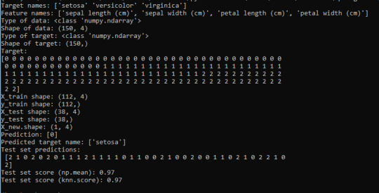
The new data I added was put into the class 0 (Setosa). And the Test set scores have a 97% accuracy score, meaning that it will be correct 97% of the time when predicting new iris flowers from new data.

My model works and it classified all of these flowers.

References

· https://docs.python.org/3/tutorial/interpreter.html

· https://unsplash.com/photos/y4xISRK8TUg

· https://en.wikipedia.org/wiki/K-nearest_neighbors_algorithm

· https://www.sas.com/en_ca/insights/analytics/machine-learning.html

· https://en.wikipedia.org/wiki/Machine_learning

· https://medium.com/gft-engineering/start-to-learn-machine-learning-with-the-iris-flower-classification-challenge-4859a920e5e3

#Youtube

0 notes

gtdk · 4 years

Text

Lasso Regression

Lasso regression is a supervised learning method. LASSO actually means Least Absolute Selection and Shrinkage Operator. Lasso imposes a constrain on the model parameters and this causes the regression variables of some coefficients to shrink towards zero. This allows to identify the variables most strongly associated with the target variable by effectively removing unimportant variables from the model.

Let’s try to implement a lasso regression model with python step by step. We will be using diabetes data set of scikit-learn.

1. Split your dataset into train and test sets. You can easily split the diabetes dataset as below.

diabetes_X, diabetes_y = datasets.load_diabetes(return_X_y=True)

X_train = diabetes_X[:-20]

X_test = diabetes_X[-20:]

y_train = diabetes_y[:-20]

y_test = diabetes_y[-20:]

2. Next we can create an object called model that will contain the results of the lasso regression. In parenthesis cv = 10 is added which askes python to use k-fold cross validation with 10 random folds from the training dataset to choose the final statistical model. To fit the lasso regression on the training set we use .fit.

from sklearn.linear_model import LassoLarsCV

model=LassoLarsCV(cv=10, precompute=False).fit(X_train,y_train)

3. Next let’s go ahead and ask python to print the regression coefficients from the model.

model.coef_

output:

array([ 0. , -194.57937837, 514.33452188, 302.88969517, -101.37105587, 0. , -234.57718479, 0. , 498.24639338, 66.14806771])

As you can see 3 coefficients have shrunk to zeros interpreting that they are unimportant variables. These variables are age,s2 and s4. Also the body mass index and the 5th blood serum has the highest coefficients.

4. Now we can plot the relative importance of the predictor selected at any step of the selection process and how the coefficients changed with addition to new variable and at which step that new variable entered the model.

import numpy as np

# plot coefficient progression

m_log_alphas = -np.log10(model.alphas_)

ax = plt.gca()plt.plot(m_log_alphas, model.coef_path_.T)

plt.axvline(-np.log10(model.alpha_), linestyle='--', color='k', label='alpha CV')

plt.ylabel('Regression Coefficients')

plt.xlabel('-log(alpha)')

plt.title('Regression Coefficients Progression for Lasso Paths')

Here the green line represents the body mass index which has the highest regression coefficient value. The yellow line is the s5.

5. Another important plot is the one that shows the changes in mean square error when the penalty parameter alpha change at each step.

# plot mean square error for each fold

m_log_alphascv = -np.log10(model.cv_alphas_)

plt.figure()

plt.plot(m_log_alphascv, model.mse_path_, ':')

plt.plot(m_log_alphascv, model.mse_path_.mean(axis=-1), 'k', label='Average across the folds', linewidth=2)

plt.axvline(-np.log10(model.alpha_), linestyle='--', color='k', label='alpha CV')

plt.legend()

plt.xlabel('-log(alpha)')

plt.ylabel('Mean squared error')

plt.title('Mean squared error on each fold')

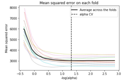
We can see that there is variability across the individual cross-validation folds in the training data set, but the change in the mean square error as variables are added to the model follows the same pattern for each fold. Initially it decreases rapidly and then levels off to a point at which adding more predictors doesn't lead to much reduction in the mean square error. This is to be expected as model complexity increases.

6. We can also print the average mean square error in the r square for the proportion of variance in school connectedness.

# MSE from training and test data

from sklearn.metrics import mean_squared_error

train_error = mean_squared_error(y_train, model.predict(X_train))

test_error = mean_squared_error(y_test, model.predict(X_test))

print ('training data MSE - ', train_error)

print ('test data MSE - ', test_error)

# R-square from training and test data

rsquared_train=model.score(X_train,y_train)

rsquared_test=model.score(X_test,y_test)

print ('training data R-square',rsquared_train)

print ('test data R-square',rsquared_test)

7. At each step of the estimation process, when a new predictor is entered into the model, the mean-square error for the validation fold is calculated for each of the other nine folds and then averaged. The model that produces the lowest mean-square error is selected by Python as the best model to validate using the test dataset.

#lassoregression python

0 notes

itsrahulpradeepposts · 4 years

Text

Why Python is used in data science? How data science courses help in a successful career post COVID pandemic?

Data science has tremendous growth opportunities and is one of the hot careers in the current world. Many businesses are thriving for skilled data scientists. Data science requires many skills to become an expert – One of the important skills is Python programming. Python is a programming language widely used in many fields. It is considered as the king of the coding world. Data scientists extensively use this language and even beginners find it easy to learn the Python language. To learn this language, there are many Python data science courses that guide and train you in an effective way.

What is Python?

Python is an interpreted and object-oriented programming language. It is an easily understandable language whose syntaxes can be grasped by a beginner quickly. It was found by Guido in 1991. It is supported in operating systems like Linux, Windows, macOS, and a lot more. The Python is developed and managed by the Python software foundation.

The second version of Python was released in 2000. It features list comprehension and reference counting. This version was officially stopped functioning in 2020. Currently, only the Python version 3.5x and later versions are supported.

Why Python is used in data science?

Python is the most preferred programming language by the data scientists as it effectively resolves tasks. It is one of the top data science tools used in various industries. It is an ideal language to implement algorithms. Python’s scikit-learn is a vital tool that the data scientist find it useful while solving many machine learning tasks. Data science uses Python libraries to solve a task.

Python is very good when it comes to scalability. It gives you flexibility and multiple solutions for different problems. It is faster than Matlab. The main reason why YouTube started working in Python is because of its exceptional scalability.

Features of Python language

Python has a syntax that can be understood easily.

It has a vast library and community support.

We can easily test codes as it has interactive modes.

The errors that arise can be easily understood and cleared quickly.

It is free software, and it can be downloaded online. Even there are free online Python compilers available.

The code can be extended by adding modules. These modules can also be implemented in other languages like C, C++, etc.

It offers a programmable interface as it is expressive in nature.

We can code Python anywhere.

The access to this language is simple. So we can easily make the program working.

The different types of Python libraries used for data science

1.Matplotlib

Matplotlib is used for effective data visualization. It is used to develop line graphs, pie charts, histograms efficiently. It has interactive features like zooming and planning the data in graphics format. The analysis and visualization of data are vital for a company. This library helps to complete the work efficiently.

2.NumPy

NumPy is a library that stands for Numerical Python. As the name suggests, it does statistical and mathematical functions that effectively handles a large n-array. This helps in improving the data and execution rate.

3.Scikit-learn

Scikit- learn is a data science tool used for machine learning. It provides many algorithms and functions that help the user through a constant interface. Therefore, it offers active data sets and capable of solving real-time problems more efficiently.

4.Pandas

Pandas is a library that is used for data analysis and manipulation. Even though the data to be manipulated is large, it does the manipulation job easily and quickly. It is an absolute best tool for data wrangling. It has two types of data structures .i.e. series, and data frame. Series takes care of one-dimensional data, and the data frame takes care of two-dimensional data.

5.Scipy

Scipy is a popular library majorly used in the data science field. It basically does scientific computation. It contains many sub-modules used primarily in science and engineering fields for FFT, signal, image processing, optimization, integration, interpolation, linear algebra, ODE solvers, etc.

Importance of data science

Data scientists are becoming more important for a company in the 21st century. They are becoming a significant factor in public agencies, private companies, trades, products and non-profit organizations. A data scientist plays as a curator, software programmer, computer scientist, etc. They are the central part of managing the collection of digital data. According to our analysis, we have listed below the major reasons why data science is important in developing the world’s economy.

Data science helps to create a relationship between the company and the client. This connection helps to know the customer’s requirements and work accordingly.

Data scientists are the base for the functioning and the growth of any product. Thus they become an important part as they are involved in doing significant tasks .i.e. data analysis and problem-solving.

There is a vast amount of data travelling around the world and if it is used efficiently, it results in the successful growth of the product.

The resulting products have a storytelling capability that creates a reliable connection among the customers. This is one of the reasons why data science is popular.

It can be applied to various industries like health-care, travel, software companies, etc.

Big data analytics is majorly used to solve the complexities and find a solution for the problems in IT companies, resource management, and human resource.

It greatly influences the retail or local sellers. Currently, due to the emergence of many supermarkets and shops, the customers approaching the retail sellers are drastically decreased. Thus data analytics helps to build a connection between the customers and local sellers.

Are you finding it difficult to answer the questions in an interview? Here are some frequently asked data science interview questions on basic concepts

Q. How to maintain a deployed model?

To maintain a deployed model, we have to

Monitor

Evaluate

Compare

Rebuild

Q. What is random forest model?

Random forest model consists of several decision trees. If you split the data into different sections and assign each group of data a decision tree, the random forest models combine all the trees.

Q. What are recommendation systems?

A recommendation system recommends the products to the users based on their previous purchases or preferences. There are mainly two areas .i.e. collaborative filtering and content-based filtering.

Q. Explain the significance of p-value?

P-value <= 0.5 : rejects the null-hypothesis

P-value > 0.5 : accepts null-hypothesis

P-value = 0.5 : it will either except or deny the null-hypothesis

Q. What is logistic regression?

Logistic regression is a method to obtain a binary result from a linear combination of predictor variables.

Q. What are the steps in building a decision tree?

Take the full data as the input.

Split the dataset in such a way that the separation of the class is maximum.

Split the input.

Follow steps 1 and 2 to the separated data again.

Stop this process after the complete data is separated.

Best Python data science courses

Many websites provide Data Science online courses. Here are the best sites that offer data science training based on Python.

GreatLearning

Coursera

EdX

Alison

Udacity

Skillathon

Konvinity

Simplilearn

How data science courses help in a successful career post-COVID-19 pandemic?

The economic downfall due to COVID-19 impacts has lead to upskill oneself as the world scenarios are changing drastically. Adding skills to your resume gives an added advantage of getting a job easily. The businesses are going to invest mainly in two domains .i.e. data analysis of customer’s demand and understanding the business numbers. It is nearly impossible to master in data science, but this lockdown may help you become a professional by indulging in data science programs.

Firstly, start searching for the best data science course on the internet. Secondly, make a master plan in such a way that you complete all the courses successfully. Many short-term courses are there online that are similar to the regular courses, but you can complete it within a few days. For example, Analytix Labs are providing these kinds of courses to upskill yourself. So this is the right time where you are free without any work and passing time. You can use this time efficiently by enrolling in these courses and become more skilled in data science than before. These course providers also give a data science certification for the course you did; this will help to build your resume.

Data science is a versatile field that has a broad scope in the current world. These data scientists are the ones who are the pillars of businesses. They use various factors like programming languages, machine learning, and statistics in solving a real-world problem. When it comes to programming languages, it is best to learn Python as it is easy to understand and has an interactive interface. Make efficient use of time in COVID-19 lockdown to upskill and build yourself.

#data science #greatlearning #python #online course #career

0 notes

your-article-is-too-long · 4 years

Text

How Does Fire Spread?

This is supplementary material for my Triplebyte blog post, “How Does Fire Spread?”

The following code creates a cellular automaton forest fire model in Python. I added so many comments to this code that the blog post became MASSIVE and the code block looked ridiculous, so I had to trim it down.

… but what if someone NEEDS it?

# The NumPy library is used to generate random numbers in the model. import numpy as np # The Matplotlib library is used to visualize the forest fire animation. import matplotlib.pyplot as plt from matplotlib import animation from matplotlib import colors # A given cell has 8 neighbors: 1 above, 1 below, 1 to the left, 1 to the right, # and 4 diagonally. The 8 sets of parentheses correspond to the locations of the 8 # neighboring cells. neighborhood = ((-1,-1), (-1,0), (-1,1), (0,-1), (0, 1), (1,-1), (1,0), (1,1)) # Assigns value 0 to EMPTY, 1 to TREE, and 2 to FIRE. Each cell in the grid is # assigned one of these values. EMPTY, TREE, FIRE = 0, 1, 2 # colors_list contains colors used in the visualization: brown for EMPTY, # dark green for TREE, and orange for FIRE. Note that the list must be 1 larger # than the number of different values in the array. Also note that the 4th entry # (‘orange’) dictates the color of the fire. colors_list = [(0.2,0,0), (0,0.5,0), (1,0,0), 'orange'] cmap = colors.ListedColormap(colors_list) # The bounds list must also be one larger than the number of different values in # the grid array. bounds = [0,1,2,3] # Maps the colors in colors_list to bins defined by bounds; data within a bin # is mapped to the color with the same index. norm = colors.BoundaryNorm(bounds, cmap.N) # The function firerules iterates the forest fire model according to the 4 model # rules outlined in the text. def firerules(X): # X1 is the future state of the forest; ny and nx (defined as 100 later in the # code) represeent the number of cells in the x and y directions, so X1 is an # array of 0s with 100 rows and 100 columns). # RULE 1 OF THE MODEL is handled by setting X1 to 0 initially and having no # rules that update FIRE cells. X1 = np.zeros((ny, nx)) # For all indices on the grid excluding the border region (which is always empty). # Note that Python is 0-indexed. for ix in range(1,nx-1): for iy in range(1,ny-1): # THIS CORRESPONDS TO RULE 4 OF THE MODEL. If the current value at # the index is 0 (EMPTY), roll the dice (np.random.random()); if the # output float value <= p (the probability of a tree being growing), # the future value at the index becomes 1 (i.e., the cell transitions # from EMPTY to TREE). if X[iy,ix] == EMPTY and np.random.random() <= p: X1[iy,ix] = TREE # THIS CORRESPONDS TO RULE 2 OF THE MODEL. # If any of the 8 neighbors of a cell are burning (FIRE), the cell # (currently TREE) becomes FIRE. if X[iy,ix] == TREE: X1[iy,ix] = TREE # To examine neighbors for fire, assign dx and dy to the # indices that make up the coordinates in neighborhood. E.g., for # the 2nd coordinate in neighborhood (-1, 0), dx is -1 and dy is 0. for dx,dy in neighborhood: if X[iy+dy,ix+dx] == FIRE: X1[iy,ix] = FIRE break # THIS CORRESPONDS TO RULE 3 OF THE MODEL. # If no neighbors are burning, roll the dice (np.random.random()); # if the output float is <= f (the probability of a lightning # strike), the cell becomes FIRE. else: if np.random.random() <= f: X1[iy,ix] = FIRE return X1 # The initial fraction of the forest occupied by trees. forest_fraction = 0.2 # p is the probability of a tree growing in an empty cell; f is the probability of # a lightning strike. p, f = 0.05, 0.001 # Forest size (number of cells in x and y directions). nx, ny = 100, 100 # Initialize the forest grid. X can be thought of as the current state. Make X an # array of 0s. X = np.zeros((ny, nx)) # X[1:ny-1, 1:nx-1] grabs the subset of X from indices 1-99 EXCLUDING 99. Since 0 is # the index, this excludes 2 rows and 2 columns (the border). # np.random.randint(0, 2, size=(ny-2, nx-2)) randomly assigns all non-border cells # 0 or 1 (2, the upper limit, is excluded). Since the border (2 rows and 2 columns) # is excluded, size=(ny-2, nx-2). X[1:ny-1, 1:nx-1] = np.random.randint(0, 2, size=(ny-2, nx-2)) # This ensures that the number of 1s in the array is below the threshold established # by forest_fraction. Note that random.random normally returns floats between # 0 and 1, but this was initialized with integers in the previous line of code. X[1:ny-1, 1:nx-1] = np.random.random(size=(ny-2, nx-2)) < forest_fraction # Adjusts the size of the figure. fig = plt.figure(figsize=(25/3, 6.25)) # Creates 1x1 grid subplot. ax = fig.add_subplot(111) # Turns off the x and y axis. ax.set_axis_off() # The matplotlib function imshow() creates an image from a 2D numpy array with 1 # square for each array element. X is the data of the image; cmap is a colormap; # norm maps the data to colormap colors. im = ax.imshow(X, cmap=cmap, norm=norm) #, interpolation='nearest') # The animate function is called to produce a frame for each generation. def animate(i): im.set_data(animate.X) animate.X = firerules(animate.X) # Binds the grid to the identifier X in the animate function's namespace. animate.X = X # Interval between frames (ms). interval = 100 # animation.FuncAnimation makes an animation by repeatedly calling a function func; # fig is the figure object used to resize, etc.; animate is the callable function # called at each frame; interval is the delay between frames (in ms). anim = animation.FuncAnimation(fig, animate, interval=interval) # Display the animated figure plt.show()

#fire #python #cellular automata #wavepropagation #forestfires #mathmodel #triplebyte

0 notes

view-from-a-warm-place · 7 years

Text

016 // Technical Notes, No.0: NumPy and Visual Effects

“Experience is something you get just after you need it.”

So I promised you a post or two ago that I would talk about some of the technical challenges and errors and misdirection I have encountered in the course of my project so far. I will try to honour that promise now!

NumPy is a set of functions and classes that mediate code written in Python, which is fairly slow in terms of processing but is easier to learn and use, with a set of its own functions written in C, which are already compiled in a way that machines can understand but are more complex and harder to write (at least as a beginner). For small data sets (containing dozens or hundreds of elements; dialogue trees, for instance, or character locations), the difference this represents is usually trivial; the time it takes to process the data in Python is not slower on an order of magnitude that humans usually notice. When the data set is large, though (thousands or millions of elements; pixel data in a graphic bitmap, in this case), it becomes a bigger deal, especially if that function runs every frame or so. (I wish I could explain this better but everything I know is self-learned and I am not a very good teacher. :/)

The waterfalls and sunbeams you may have seen here and there in Nigran Cavern and outside the shuttle wreck in Opark Forest are two places where I have used NumPy to generate graphics on-the-spot using code, rather than raw images. These elements are generated and updated entirely in code, rather than from any sort of base image or animation, and the way their geometry changes is entirely random*. This is useful for a few reasons, primarily because it frees me from having to draw and make unique every waterfall and sunbeam in every situation, and because it liberates disk space that those graphics would have otherwise taken up. The price I pay is that the software has to both generate and continuously revise the graphic elements on-the-spot, though, in addition to displaying them, which requires processing power beyond simply flipping through pre-drawn frames, and as stated, Python and Pygame are a bit stunted in this area of information processing. NumPy really helps in this area, effectively having the bitmap data array processing carried out directly by the computer hardware (rather than by way of Python’s bytecode interpreter) so that Python does not have to try, but in so doing creates new and additional problems as NumPy and Pygame do not always play nicely together.

Pygame is equipped with a module called surfarray which allows the software to directly intervene in a bitmap’s pixels; it could be a very useful tool, but the problem is that it is buggy and Pygame has not been officially supported for years. The pixels2d and pixels3d functions, which are the ones relevant to my code, create “memory leaks,” which are basically blocks of memory that the software reserves, fiddles around inside of, but then forgets to release for some reason** when it finishes with it. It does this every time I call it, which can be two or three times per frame, depending on what the player is looking at. If the software runs at thirty frames per second, it can accumulate thousands of useless bitmaps every minute, which stick around in memory until either the program closes (hopefully) or until the system runs out of memory and crashes. I found three obvious solutions: try to correct the problem directly by debugging Pygame’s surfarray code, which I did not know how to do since it was partially in C (which I also do not know much about); I could use the similar surfarray.pixels#d functions, which do the same thing but take some time to make copies of the bitmap arrays for you to edit (rather than editing pixel data in-place); or I could abandon the surfarray functions entirely and do something else, which partially became my solution.

What I ended up doing was leaving the pixels#d functions alone, but trying out the thankfully-not-buggy pixels_alpha function, which works solely with an image’s transparency channel. It turns out that bumping opacity around is more than enough to create a decent-looking waterfall (water is all the same colour anyway, right?) without worrying too much, and since the function avoided the problems its companions fell victim to, I ended up going with that. Admittedly, there remain issues: Pygame can only handle the effect element as 32-bit surfaces (wherein each pixel has a value for a red, green, blue, and opacity channel) even though the only channel that actually bears any contrast is the opacity value (the red, green, and blue values are identical for all pixels), which means that 24 bits of data on each pixel could be effectively described by a single value for the entire image (which is a bunch of wasted memory), for one; also, pixels_alpha works without hazard on my computer and with my version of Pygame, but it may not be so cooperative on other systems– a degree of compatibility I would not worry about if the library it came from was more reliable.

The sunbeams in Opark and in the Nigran Cavern Entryway are generated in a similar way.

As I said in post 014 though, I do not really look down on them for their technical ‘inadequacies’, because they seem pleasant to look at and are not excessively demanding processor-wise. The entire project remains as it was when I began: experimental, and I think that this aspect of it makes it especially enjoyable to develop. Also, what else could you call something created by someone who started with no idea of what they were doing?

Anyway, that is all for this week’s post. Depending on how well map development goes between now and the next entry, I may have some images for you next week, or maybe I might go over some tileset stuff. Post a reply to this entry if you have some preference one way or the other, or maybe for a third thing! :D

See you next week~

* In the extent that the meta-random values Python's native `random` library can be "entirely random."

** As near as I can figure, Python’s garbage collection never clears them out because they create some internal reference that they never got around to breaking when the pixels#d output array is ‘orphaned’. But I what I do not know about Pygame could fill a wharf’s worth of warehouses. :/

#longpost #pygame #python #numpy #inform #props #assets #nigran cavern #opark forest #animat #development #visual aesthetic #tech #visual effects

2 notes · View notes

rafi1228 · 5 years

Link

The Numpy, Scipy, Pandas, and Matplotlib stack: prep for deep learning, machine learning, and artificial intelligence

What you’ll learn

Understand supervised machine learning (classification and regression) with real-world examples using Scikit-Learn

Understand and code using the Numpy stack

Make use of Numpy, Scipy, Matplotlib, and Pandas to implement numerical algorithms

Understand the pros and cons of various machine learning models, including Deep Learning, Decision Trees, Random Forest, Linear Regression, Boosting, and More!

Requirements

Understand linear algebra and the Gaussian distribution

Be comfortable with coding in Python

You should already know “why” things like a dot product, matrix inversion, and Gaussian probability distributions are useful and what they can be used for

Description

Welcome! This is Deep Learning, Machine Learning, and Data Science Prerequisites: The Numpy Stack in Python.

One question or concern I get a lot is that people want to learn deep learning and data science, so they take these courses, but they get left behind because they don’t know enough about the Numpy stack in order to turn those concepts into code.

Even if I write the code in full, if you don’t know Numpy, then it’s still very hard to read.

This course is designed to remove that obstacle – to show you how to do things in the Numpy stack that are frequently needed in deep learning and data science.

So what are those things?

Numpy. This forms the basis for everything else. The central object in Numpy is the Numpy array, on which you can do various operations.

The key is that a Numpy array isn’t just a regular array you’d see in a language like Java or C++, but instead is like a mathematical object like a vector or a matrix.

That means you can do vector and matrix operations like addition, subtraction, and multiplication.

The most important aspect of Numpy arrays is that they are optimized for speed. So we’re going to do a demo where I prove to you that using a Numpy vectorized operation is faster than using a Python list.

Then we’ll look at some more complicated matrix operations, like products, inverses, determinants, and solving linear systems.

Pandas. Pandas is great because it does a lot of things under the hood, which makes your life easier because you then don’t need to code those things manually.

Pandas makes working with datasets a lot like R, if you’re familiar with R.

The central object in R and Pandas is the DataFrame.

We’ll look at how much easier it is to load a dataset using Pandas vs. trying to do it manually.

Then we’ll look at some dataframe operations, like filtering by column, filtering by row, the apply function, and joins, which look a lot like SQL joins.

So if you have an SQL background and you like working with tables then Pandas will be a great next thing to learn about.

Since Pandas teaches us how to load data, the next step will be looking at the data. For that we will use Matplotlib.

In this section we’ll go over some common plots, namely the line chart, scatter plot, and histogram.

We’ll also look at how to show images using Matplotlib.

99% of the time, you’ll be using some form of the above plots.

Scipy.

I like to think of Scipy as an addon library to Numpy.

Whereas Numpy provides basic building blocks, like vectors, matrices, and operations on them, Scipy uses those general building blocks to do specific things.

For example, Scipy can do many common statistics calculations, including getting the PDF value, the CDF value, sampling from a distribution, and statistical testing.

It has signal processing tools so it can do things like convolution and the Fourier transform.

In sum:

If you’ve taken a deep learning or machine learning course, and you understand the theory, and you can see the code, but you can’t make the connection between how to turn those algorithms into actual running code, this course is for you.

HARD PREREQUISITES / KNOWLEDGE YOU ARE ASSUMED TO HAVE:

linear algebra

probability

Python coding: if/else, loops, lists, dicts, sets

you should already know “why” things like a dot product, matrix inversion, and Gaussian probability distributions are useful and what they can be used for

TIPS (for getting through the course):

Watch it at 2x.

Take handwritten notes. This will drastically increase your ability to retain the information. This has been proven by research!

Ask lots of questions on the discussion board. The more the better!

Realize that most exercises will take you days or weeks to complete.

WHAT ORDER SHOULD I TAKE YOUR COURSES IN?:

Check out the lecture “What order should I take your courses in?” (available in the Appendix of any of my courses)

Who this course is for:

Students and professionals with little Numpy experience who plan to learn deep learning and machine learning later

Students and professionals who have tried machine learning and data science but are having trouble putting the ideas down in code

Created by Lazy Programmer Inc. Last updated 3/2019 English English [Auto-generated]

Size: 852.70 MB

Download Now

https://ift.tt/2fu80Fd.

The post Deep Learning Prerequisites: The Numpy Stack in Python appeared first on Free Course Lab.

#IFTTT #Blogger

0 notes

manojmme-blog · 5 years

Text

MACHINE LEARNING TRAINING IN VIJAYAWADA

Machine Learning Course

Machine Learning is a set of algorithms that help the machines, that is the computers, devices, and every bit of technology that uses Artificial Intelligence to ‘learn’ from their own experiences with varying amount of human intervention. Some Machine Learning algorithms need humans to modify their codes regularly while others can modify the algorithms themselves. Machine Learning training can enable a person to code such algorithms which would be able to process large data and use the result to modify itself, make future predictions, mimic human behavior, and many such activities. Every year millions of dollars are spent on developing new algorithms for Machine Learning in order to help companies increase their efficiency and productivity. Having a Machine Learning certification would help software engineers to tap into this market.

Using Machine Learning in Numerous Industries

At Codegnan, we provide one of the best Machine Learning training in Vijayawada. Machine Learning is truly transforming numerous industries by revolutionizing the processes of manufacturing and production, sales and purchases, marketing, communication, cybersecurity, and basically every aspect of an organization. A Machine Learning training course allows you to understand the important roles that the data scientist and Machine Learning engineer play in today’s data-savvy environment. Let’s look at all the various industries that you will be able to get into after taking a Machine Learning course:

Manufacturing: Machine Learning training institutes like us also teach you to use Machine Learning algorithms to ease the process of manufacturing, increase efficiency and productivity, and reduce the need for human labor. This can be achieved by training the algorithm to carry out the manufacturing processes, find flaws in them and to modify the process based on the limitations.

Stock Market: One of the extensive parts in Machine Learning training is writing algorithms that can collect a large amount of data from various sources, analyze it to understand the relationship between them and their past trends in order to predict the future trends. This can be used to predict the stock market trends by using Machine Learning and thus as a way to make profitable trades.

Cybersecurity: Every day there are millions of new cyber attacks carried out on people all around the world which leads to huge losses of protected data as well as money globally. Cyber attacks on organizations and their employees can lead to devastating consequences and disrupt their working for a significant amount of time. This is why cyber attacks have been recognized as one of the most harmful threats worldwide. The worst part about cyber attacks is that the attackers keep on developing their codes which is why traditional methods of cybersecurity are not enough. Machine Learning algorithms can be used to store information of the past codes of cyber attacks, detect the patterns in them, and use them to detect any future malicious code with as much as 2% to 10% variation in coding. Thus, Machine Learning can drastically change the cybersecurity industry.

E-Commerce: The Machine Learning course also includes learning how to use Machine Learning to help an eCommerce business. The algorithms can be designed to collect all the data and analyze it to ascertain the shopping patterns and product preferences of the consumers. With the help of this analysis, it can further understand the psychology of people while shopping and use it to improve their shopping experience, conversion rates, and recommend relevant products to the users. It also helps in the targeted advertisement. Many Others: After taking Machine Learning training course from us you will be able to use your knowledge of Machine Learning for a plethora of other purposes as well. For example, creating virtual personal assistants, social media services, predicting trends for various purposes such as while commuting, video surveillance, developing virtual customer support, refining search engine results, and much more.

Why CodeGnan to be chosen to learn Machine Learning training in Vijayawada?

Codegnan provides over 60 hours of the best course in machine learning training in Vijayawada. This course is further divided into several parts to ensure that you have the proper understanding of each of the part before proceeding to the next level. Being one of the premier Machine Learning training institutes we provide you with the opportunity to work on real-life case studies with the leading Machine Learning engineers and scientists as a hands-on approach for teaching. By the end of the course, you would be able to write supervised and unsupervised algorithms to carry out various tasks and to modify themselves based on the available data.

CURRICULUM

Course Syllabus

Part 1 Introduction to Python. Who is using Python today? Installation and setting up environment. Basic syntax. Built in data types.

Part 2 Basic Operators. Decision making. Loops. Numbers. Strings. Lists.

Part 3 Tuples. Sets. Dictionary. Functions. Modules.

Part 4 Packages. Files. Exceptions. Classes. Regular Expressions.

Part 5 Database Access. Networking. Sending Email. Building Microservices. Working with git.

Part 6 Numpy. Multi-dimensional array. Files with arrays. Linear Algebra. Array Manipulation. Structured and record arrays.

Part 7 Pandas. Series. Data Frames. Reading and Writing Data in Text Format.

Part 8 Interacting with web APIs. Interacting with Databases. Handling missing data. Combining and merging datasets.

Part 9 Matplotlib. Plotting and visualizing data. Data aggregation. Time series. Time zones. Sickit learn.

Part 10 Introduction to Machine Learning How do machines learn Types of machine learning Supervised learning Unsupervised learning Reinforcement learning

Applications of machine learning

Part 11 Selecting a model Training a model Classification Regression Clustering Performance of a model

Part 12 What is a feature Feature construction Feature extraction Feature selection

Part 13 Supervised learning classification. Bayes Theorem Naïve Bayes Classifier K-Nearest Neighbour (KNN) Decision Tree. Random Forest Model Support Vector Machines

Part 14 Supervised learning regression. Simple linear regression. Multiple linear regression. Problems in regression analysis. Polynomial regression model. Logistic Regression.

Part 15 Unsupervised vs Supervised learning. Applications of Unsupervised Learning Clustering

#machine learning #machine learning training in vijayawada #codegnan

0 notes

rohithgo-blog · 5 years

Text

MACHINE LEARNING TRAINING IN VIJAYAWADA

Machine Learning Course

Using Machine Learning in Numerous Industries At Codegnan, we provide one of the best Machine Learning training in Vijayawada. Machine Learning is truly transforming numerous industries by revolutionizing the processes of manufacturing and production, sales and purchases, marketing, communication, cybersecurity, and basically every aspect of an organization. A Machine Learning training course allows you to understand the important roles that the data scientist and Machine Learning engineer play in today’s data-savvy environment. Let’s look at all the various industries that you will be able to get into after taking a Machine Learning course:

Healthcare: Healthcare industry is one of the most profitable industries around the world. Here every new innovation can earn you hundreds of millions of dollars. By and by healthcare industry is adopting more IoT and other connected devices. With a Machine Learning certification, you will be able to code Machine Learning algorithms to track the patients’ health, collect data, analyze it, and predict future health trends. It helps the devices to alert the healthcare providers in case the patients’ health shows signs of deteriorating. Manufacturing: Machine Learning training institutes like us also teach you to use Machine Learning algorithms to ease the process of manufacturing, increase efficiency and productivity, and reduce the need for human labor. This can be achieved by training the algorithm to carry out the manufacturing processes, find flaws in them and to modify the process based on the limitations. Stock Market: One of the extensive parts in Machine Learning training is writing algorithms that can collect a large amount of data from various sources, analyze it to understand the relationship between them and their past trends in order to predict the future trends. This can be used to predict the stock market trends by using Machine Learning and thus as a way to make profitable trades. Cybersecurity: Every day there are millions of new cyber attacks carried out on people all around the world which leads to huge losses of protected data as well as money globally. Cyber attacks on organizations and their employees can lead to devastating consequences and disrupt their working for a significant amount of time. This is why cyber attacks have been recognized as one of the most harmful threats worldwide. The worst part about cyber attacks is that the attackers keep on developing their codes which is why traditional methods of cybersecurity are not enough. Machine Learning algorithms can be used to store information of the past codes of cyber attacks, detect the patterns in them, and use them to detect any future malicious code with as much as 2% to 10% variation in coding. Thus, Machine Learning can drastically change the cybersecurity industry. E-Commerce: The Machine Learning course also includes learning how to use Machine Learning to help an eCommerce business. The algorithms can be designed to collect all the data and analyze it to ascertain the shopping patterns and product preferences of the consumers. With the help of this analysis, it can further understand the psychology of people while shopping and use it to improve their shopping experience, conversion rates, and recommend relevant products to the users. It also helps in the targeted advertisement. Many Others: After taking Machine Learning training course from us you will be able to use your knowledge of Machine Learning for a plethora of other purposes as well. For example, creating virtual personal assistants, social media services, predicting trends for various purposes such as while commuting, video surveillance, developing virtual customer support, refining search engine results, and much more. Why CodeGnan to be chosen to learn Machine Learning training in Vijayawada? Codegnan provides over 60 hours of the best course in machine learning training in Vijayawada. This course is further divided into several parts to ensure that you have the proper understanding of each of the part before proceeding to the next level. Being one of the premier Machine Learning training institutes we provide you with the opportunity to work on real-life case studies with the leading Machine Learning engineers and scientists as a hands-on approach for teaching. By the end of the course, you would be able to write supervised and unsupervised algorithms to carry out various tasks and to modify themselves based on the available data.

CURRICULUM Course Syllabus Z Part 1 Introduction to Python. Who is using Python today? Installation and setting up environment. Basic syntax. Built in data types. Z Part 2 Basic Operators. Decision making. Loops. Numbers. Strings. Lists. Z Part 3 Tuples. Sets. Dictionary. Functions. Modules. Z Part 4 Packages. Files. Exceptions. Classes. Regular Expressions. Z Part 5 Database Access. Networking. Sending Email. Building Microservices. Working with git. Z Part 6 Numpy. Multi-dimensional array. Files with arrays. Linear Algebra. Array Manipulation. Structured and record arrays. Z Part 7 Pandas. Series. Data Frames. Reading and Writing Data in Text Format. Z Part 8 Interacting with web APIs. Interacting with Databases. Handling missing data. Combining and merging datasets. Z Part 9 Matplotlib. Plotting and visualizing data. Data aggregation. Time series. Time zones. Sickit learn. Z Part 10 Introduction to Machine Learning How do machines learn Types of machine learning Supervised learning Unsupervised learning Reinforcement learning

Applications of machine learning

Z Part 11 Selecting a model Training a model Classification Regression Clustering Performance of a model Z Part 12 What is a feature Feature construction Feature extraction Feature selection Z Part 13 Supervised learning classification. Bayes Theorem Naïve Bayes Classifier K-Nearest Neighbour (KNN) Decision Tree. Random Forest Model Support Vector Machines Z Part 14 Supervised learning regression. Simple linear regression. Multiple linear regression. Problems in regression analysis. Polynomial regression model. Logistic Regression. Z Part 15 Unsupervised vs Supervised learning. Applications of Unsupervised Learning Clustering

#machine learning #machine learning training in vijayawada #codegnan

0 notes