#exog | Explore Tumblr posts and blogs

adaleecrypto · 1 year ago

Text

Panel VAR in Stata and PVAR-DY-FFT

Preparation

xtset pros mm (province, month)

Endogenous variables:

global Y loan_midyoy y1 stock_pro

Provincial medium-term loans year-on-year (%)

Provincial 1-year interest rate (%) (NSS model estimate, not included in this article) (%)

provincial stock return

Exogenous variables:

global X lnewcasenet m2yoy reserve_diff

Logarithm of number of confirmed cases

M2 year-on-year

reserve ratio difference

Descriptive statistics:

global V loan_midyoy y1 y10 lnewcasenet m2yoy reserve_diff sum2docx $V using "D.docx", replace stats(N mean sd min p25 median p75 max ) title("Descriptive statistics")

VarName Obs Mean SD Min P25 Median P75 Max

loan_midyoy 2232 13.461 7.463 -79.300 9.400 13.400 16.800 107.400

y1 2232 2.842 0.447 1.564 2.496 2.835 3.124 4.462

stock_pro 2232 0.109 6.753 -24.485 -3.986 -0.122 3.541 73.985

lnewcasenet 2232 1.793 2.603 0.000 0.000 0.000 3.434 13.226

m2yoy 2232 0.095 0.012 0.080 0.085 0.091 0.105 0.124

reserve_diff 2232 -0.083 0.232 -1.000 0.000 0.000 0.000 0.000

Check for unit root：

foreach x of global V { xtunitroot ips `x',trend }

Lag order

pvarsoc $Y , pinstl(1/5)

pvaro(instl(4/8)): Specifies to use the fourth through eighth lags of each variable as instrumental variables. In this case, in order to deal with endogeneity issues, relatively distant lags are chosen as instrumental variables. This means that when estimating the model, the current value of each variable is not directly affected by its own recent lagged value (first to third lag), thus reducing the possibility of endogeneity.

pinstl(1/5): Indicates using lags from the highest lag to the fifth lag as instrumental variables. Specifically, for the PVAR(1) model, the first to fifth lags are used as instrumental variables; for the PVAR(2) model, the second to sixth lags are used as instrumental variables, and so on. The purpose of this approach is to provide each model variable with a set of instrumental variables that are related to, but relatively independent of, its own lag structure, thereby helping to address endogeneity issues.

CD test (Cross-sectional Dependence Test): This is a test to detect whether there is cross-sectional dependence (ie, correlation between different individuals) in panel data. Values close to 1 generally indicate the presence of strong cross-sectional dependence. If there is cross-sectional dependence in the data, cluster-robust standard errors can be used to correct for this.

J-statistic: The J-statistic that detects model over-identification of constraints and is usually related to the effectiveness of instrumental variables.

J pvalue: The p value of the J statistic, used to determine whether the instrumental variable is valid. A low p-value (usually less than 0.05) means that at least one of the instrumental variables is probably not applicable.

MBIC, MAIC, MQIC: These are different information criterion values, used for model selection. Lower values generally indicate a better model.

MBIC: Bayesian Information Criterion.

MAIC: Akaike Information Criterion.

MQIC: Quantile information criterion.

Interpretation: The p-values of the J-test are 0.00 and 0.63 for Lag 1 and Lag 2 respectively. The p-value for the first lag is very low, indicating possible instrumental variable inefficiency. The p-value for the second lag is higher, indicating that instrumental variables may be effective. In this example, Lag 2 seems to be the optimal choice because its MBIC, AIC, and MQIC values are relatively low. However, it should be noted that the CD test shows that there is cross-sectional dependence, which may affect the accuracy of model estimation.

Model estimation：

pvar $Y, lags(2) instlags(1/4) fod exog($X) gmmopts(winitial(identity) wmatrix(robust) twostep vce(cluster pros))

pvar: This is the Stata command that calls the PVAR model.

$Y: These are the endogenous variables included in the model.

$X: These are exogenous variables included in the model.

lags(2): Specifies to include 2-period lags for each variable in the PVAR model.

number of lag periods for the variable

instlags(1/4): This is the number of lags for the specified instrumental variable. Here, it tells Stata to use the first to fourth lags as instrumental variables. This is to address possible endogeneity issues, i.e. possible interactions between variables in the model.

Lag order selection criteria:

Information criterion: Statistical criteria such as AIC and BIC can be used to judge the choice of lag period.

Diagnostic tests: Use diagnostic tests of the model (e.g. Q(b), Hansen J overidentification test) to assess the appropriateness of different lag settings.

fod/fd: medium fixed effects.

fod: The Helmert transformation is a forward mean difference method that compares each observation to the mean of its future observations. This method makes more efficient use of available information than simple difference-in-difference methods when dealing with fixed effects, especially when the time dimension of panel data is short.

A requirement of the Helmert transformation on the data is that the panel must be balanced (i.e., for each panel unit, there are observations at all time points).

fd: Use first differences to remove panel-specific fixed effects. In this method, each observation is subtracted from its observation in the previous period, thus eliminating the influence of time-invariant fixed effects. First difference is a common method for dealing with fixed effects in panel data, especially when there is a trend or horizontal shift in the data over time.

Usage Scenarios and Choices: If your panel data is balanced and you want to utilize time series information more efficiently, you may be inclined to use the Helmert transformation. First differences may be more appropriate if the data contain unbalanced panels or if there is greater concern with removing possible time trends and horizontal shifts.

exog($X): This option is used to specify exogenous variables in the model. Exogenous variables are assumed to be variables that are not affected by other variables in the model.

gmmopts(winitial(identity) wmatrix(robust) twostep vce(cluster pros))

winitial(identity): Set the initial weight matrix to the identity matrix.

wmatrix(robust): Use a robust weight matrix.

twostep: Use the two-step GMM estimation method.

vce(cluster pros): Specifies the standard error of clustering robustness, and uses `pros` as the clustering variable.

GMM criterion function

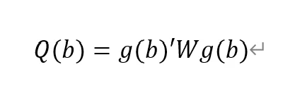
Final GMM Criterion Q(b) = 0.0162: The GMM criterion function (Q(b)) is a mathematical expression that measures how consistent your model parameter estimates (b) are with these moment conditions. Simply put, it measures the gap between model parameters and theoretical or empirical expectations.

is a vector of moment conditions. These moment conditions are a series of assumptions or constraints set based on the model. They usually come in the form of expected values (expectations) that represent the conditions that the model parameter b should satisfy.

W is a weight matrix used to assign different weights to different moment conditions.

b is a vector of model parameters. The goal of GMM estimation is to find the optimal b to minimize Q(b).

No. of obs = 2077: This means there are a total of 2077 observations in the data set.

No. of panels = 31: This means that the data set contains 31 panel units.

Ave. no. of T = 67.000: Each panel unit has an average of 67 time point observations.

Coefficient interpretation (not marginal effects)

L1.loan_midyoy: 0.8034088: When the one-period lag of loan_midyoy increases by one unit, the current period's loan_midyoy is expected to increase by approximately 0.803 units. This coefficient is statistically significant (p-value 0.000), indicating that the one-period lag has a significant positive impact on the current value.

L2.loan_midyoy: 0.1022556: When the two-period lag of loan_midyoy increases by one unit, the current period's loan_midyoy is expected to increase by approximately 0.102 units. This coefficient is not statistically significant (p-value of 0.3), indicating that the effect of the two-period lag on the current value may not be significant.

overidentification test

pvar $Y, lags(2) instlags(1/4) fod exog($X) gmmopts(winitial(identity) wmatrix(robust) twostep vce(cluster pros)) overid (written in one line)

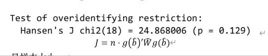
Statistics: Hansen's J chi2(18) = 24.87 means that the chi-square statistic value of the Hansen J test is 24.87 and the degrees of freedom are 18.

P-value: (p = 0.137) means that the p-value of this test is 0.129. Since the p-value is higher than commonly used significance levels (such as 0.05 or 0.01), this indicates that there is insufficient evidence to reject the null hypothesis. In the Hansen J test, the null hypothesis is that all instrumental variables are exogenous, that is, they are uncorrelated with the error term. Instrumental variables may be appropriate.

Stability check:

pvarstable

Eigenvalues: Listed eigenvalues include their real and imaginary parts. For example, 0.9271743 is a real eigenvalue. 0.0337797±0.326651i is a pair of conjugate complex eigenvalues.

Modulus: The module of an eigenvalue is its distance from the origin on the complex plane. It is calculated as the square root of the sum of the squares of the real and imaginary parts.

Stability condition: The stability condition of the PVAR model requires that the modules of all eigenvalues must be less than or equal to 1 (that is, all eigenvalues are located within the unit circle).

Granger causality:

pvargranger

Ho (null hypothesis): The excluded variable is not a Granger cause (i.e. does not have a predictive effect on the variables in the equation).

Ha (alternative hypothesis): The excluded variable is a Granger cause (i.e. has a predictive effect on the variables in the equation).

For the stock_pro equation:

loan_midyoy: chi2 = 6.224 (degrees of freedom df = 2), p-value = 0.045. There is sufficient evidence to reject the null hypothesis, indicating that loan_midyoy is the Granger cause of stock_pro.

y1: chi2 = 0.605 (degrees of freedom df = 2), p-value = 0.739. There is insufficient evidence to reject the null hypothesis indicating that y1 is not the Granger cause of stock_pro.

Margins:

The PVAR model involves the dynamic interaction of multiple endogenous variables, which means that the current value of a variable is not only affected by its own past values, but also by the past values of other variables. In this case, the margins command may not be suitable for calculating or interpreting the marginal effects of variables in the model, because these effects are not fixed but change dynamically with time and the state of the model. The following approaches may be considered:

Impulse response analysis

Impulse response analysis: In the PVAR model, the more common analysis method is to perform impulse response analysis (Impulse Response Analysis), which can help understand how the impact of one variable affects other variables in the system over time.

pvarirf,oirf mc(200) tab

Orthogonalized Impulse Response Function (OIRF): In some economic or financial models, orthogonalized processing may be more realistic, especially when analyzing policy shocks or other clearly distinguished externalities. During impact. If the shocks in the model are assumed to be independent of each other, then OIRF should be used. Orthogonalization ensures that each shock is orthogonal (statistically independent) through a mathematical process (such as Cholisky decomposition). This means that the effect of each shock is calculated controlling for the other shocks.

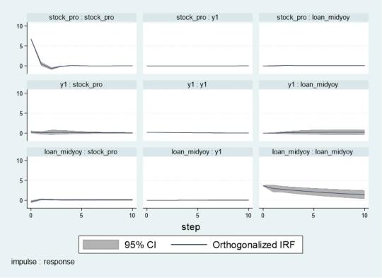
When stock_pro is subject to a positive shock of one standard deviation, loan_midyoy is expected to decrease slightly in the first period, with a specific response value of -0.0028833, indicating that loan_midyoy is expected to decrease by approximately 0.0029 units.

This effect gradually changes over time. For example, in the second period, the shock response of loan_midyoy to stock_pro is 0.0700289, which means that loan_midyoy is expected to increase by about 0.0700 units.

pvarirf, mc(200) tab

For some complex dynamic systems, non-orthogonalized IRF may be better able to capture the actual interactions between variables within the system. Non-orthogonalized impulse response function: If you do not make the assumption that the shocks are independent of each other, or if you believe that there is some inherent interdependence between the variables in the model, you may choose a non-orthogonalized IRF.

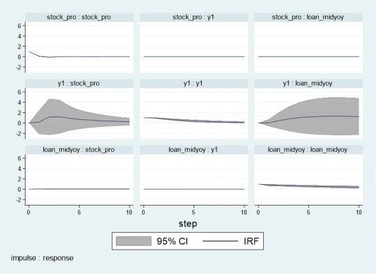
When stock_pro is impacted: In period 1, loan_midyoy has a slightly negative response to the impact on stock_pro, with a response value of -0.0004269.

This effect gradually changes over time. For example, in period 2, the response value is 0.0103697, indicating that loan_midyoy is expected to increase slightly.

Forecast error variance decomposition

Forecast Error Variance Decomposition is also a useful tool for analyzing the dynamic relationship between variables in the PVAR model.

Time point 0: The contribution of all variables is 0, because at the initial moment when the impact occurs, no variables have an impact on loan_midyoy.

Time point 1: The forecast error variance of loan_midyoy is completely explained by its own shock (100%), while the contribution of y1 and stock_pro is 0.

Subsequent time points: For example, at time point 10, about 99.45% of the forecast error variance of loan_midyoy is explained by the shock to loan_midyoy itself, about 0.52% is explained by the shock to y1, and about 0.03% is explained by the shock to stock_pro.

Diebold-Yilmaz (DY) variance decomposition

Diebold-Yilmaz (DY) variance decomposition is an econometric method used to quantify volatility spillovers between variables in time series data. This approach is based on the vector autoregressive (VAR) model, which is used particularly in the field of financial economics to analyze and understand the interaction between market variables. The following are the key concepts of DY variance decomposition:

basic concepts

VAR model: The VAR model is a statistical model used to describe the dynamic relationship between multiple time series variables. The VAR model assumes that the current value of each variable depends not only on its own historical value, but also on the historical values of other variables.

Forecast error variance decomposition (FEVD): In the VAR model, FEVD analysis is used to determine what proportion of the forecast error of a variable can be attributed to the impact of other variables.

Volatility spillover index: The volatility spillover index proposed by Diebold and Yilmaz is based on FEVD, which quantifies the contribution of the fluctuation of each variable in a system to the fluctuation of other variables.

"From" and "to" spillover: DY variance decomposition distinguishes between "from" and "to" spillover effects. "From" spillover refers to the influence of a certain variable on the fluctuation of other variables in the system; while "flow to" spillover refers to the influence of other variables in the system on the fluctuation of that specific variable.

Application

Financial market analysis: DY variance decomposition is particularly important in financial market analysis. For example, it can be used to analyze the fluctuation correlation between stock markets in different countries, or the extent of risk spillovers during financial crises.

Policy evaluation: In macroeconomic policy analysis, DY analysis can help policymakers understand the impact of policy decisions (such as interest rate changes) on various areas of the economy.

Precautions

Explanation: DY analysis provides a way to quantify volatility spillover, but it cannot be directly interpreted as cause and effect. The spillover index reflects correlation, not causation, of fluctuations.

Model setting: The effectiveness of DY analysis depends on the correct setting of the VAR model, including the selection of variables, the determination of the lag order, etc.

mat list e(Sigma)

mat list e(b)

Since I have previously made a DY model suitable for variable coefficients, I only need to fill in the time-varying coefficients in the first period. Because when there is only one period, the results of the constant coefficient and the variable coefficient are the same.

Since stata does not have the original code of dy, R has the spillover package, which can be modified without errors. Therefore, the spillover package of R language is recommended. It is taken from the code in bk2018 article.

Therefore, you need to manually fill in the stata coefficients into the interface part I made in R language, and then continue with the BK code.

```{r} library(tvpfft) library(tvpgevd) library(tvvardy) library(ggplot2) library(gridExtra) a = rbind(c(0,.80340884 , .02610899, -.00042695, .10225563, .39926325, .01073319 ), c(0, .00269745, .97914619, .00044023, .00063315, -.16136799, -.00038024), c(0, .06798046, .1483059 , .07497919, -.02856828, 1.0076676, -.10757831)) ``` ```{r} Sigma = rbind(c( 13.495069, .01625753, -1.3143064), c( .01625753, .03064462, .04350408 ), c( -1.3143064, .04350408, 45.800811)) df=data.frame(t(c(1,1,1))) colnames(df)=c("loan_midyoy","y1","stock_pro") fit = list() fit$Beta.postmean=array(dim =c(3,7,1)) fit$H.postmean=array(dim =c(3,3,1)) fit$Beta.postmean[,,1]=a fit$H.postmean[,,1]=Sigma fit$M=3tvp.gevd(fit, 37, df) ```

Diagonal line (loan_midyoy vs. loan_midyoy, y1 vs. y1, stock_pro vs. stock_pro): shows that the main source of fluctuations in each variable is its own fluctuation. For example, 98.52% of loan_midyoy's fluctuations are caused by itself.

Off-diagonal lines (such as the y1 and stock_pro rows of the loan_midyoy column): represent the contribution of other variables to the loan_midyoy fluctuations. In this example, y1 and stock_pro contribute very little to the fluctuation of loan_midyoy, 1.37% and 0.11% respectively.

The "From" row: shows the overall contribution of each variable to the fluctuations of all other variables. For example, the total contribution of loan_midyoy to the fluctuation of all other variables in the system is 0.49%.

"To" column: reflects the overall contribution of all other variables in the system to the fluctuation of a single variable. For example, the total contribution of other variables in the system to the fluctuation of loan_midyoy is 5.30%.

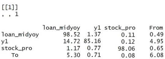
Analysis and interpretation:

Self-contribution: The fluctuations of loan_midyoy, y1, and stock_pro are mainly caused by their own shocks, which can be seen from the high percentages on their diagonals.

Mutual influence: y1 and stock_pro contribute less to each other's fluctuations, but y1 has a relatively large contribution to the fluctuations of loan_midyoy (14.72%).

System Fluctuation Impact: The “From” and “To” columns provide an overall measure of spillover effects. For example, stock_pro has a small contribution to the fluctuation of the system (0.65% comes from the impact of stock_pro), but the system has a greater impact on the fluctuation of stock_pro (6.08% of the fluctuation comes from the system).```{r} tvp.gevd.fft(fit, df, c(pi+0.00001,pi/12,0),37) ```

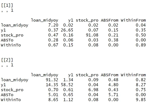
The same goes for Fourier transform. It is divided into those within 1 year and 1-3 years, and the sum is the previous picture.

DY I used the R language's spillover package to modify the interface.

Part of the code logic:

function (ir1, h, Sigma, df) { ir10 <- list() n <- length(Sigma[, 1]) for (oo in 1:n) { ir10[[oo]] <- matrix(ncol = n, nrow = h) for (pp in 1:n) { rep <- oo + (pp - 1) * (n) ir10[[oo]][, pp] <- ir1[, rep] } } ir1 <- lapply(1:(h), function(j) sapply(ir10, function(i) i[j, ])) denom <- diag(Reduce("+", lapply(ir1, function(i) i %*% Sigma %*% t(i)))) enum <- Reduce("+", lapply(ir1, function(i) (i %*% Sigma)^2)) tab <- sapply(1:nrow(enum), function(j) enum[j, ]/(denom[j] * diag(Sigma))) tab0 <- t(apply(tab, 2, function(i) i/sum(i))) assets <- colnames(df) n <- length(tab0[, 1]) stand <- matrix(0, ncol = (n + 1), nrow = (n + 1)) stand[1:n, 1:n] <- tab0 * 100 stand2 <- stand - diag(diag(stand)) stand[1:(n + 1), (n + 1)] <- rowSums(stand2)/n stand[(n + 1), 1:(n + 1)] <- colSums(stand2)/n stand[(n + 1), (n + 1)] <- sum(stand[, (n + 1)]) colnames(stand) <- c(colnames(df), "From") rownames(stand) <- c(colnames(df), "To") stand = round(stand, 2) return(stand) }

#Panel VAR #stata #R #Econometrics

0 notes