#strouhal
Explore tagged Tumblr posts
Visit Tumblr Blog
Explore Tumblr blogs with no restrictions, modern design and the best experience.
Last Seen Tumblr Blogs


Fun Fact
Total funding amounts to $125.3M.
Text
My clit is aerodynamic as hell and would not be caught dead shedding vortices like that, even at very high Strouhal number
I bet that your clit cannot even do this !
6K notes
·
View notes
Text
Die Kunst des Blätterns – Verzetteltes Schreiben, zerstreutes Lesen
Das Blättern ist eine Geste. Eine Bewegung, die sich scheinbar beiläufig vollzieht, deren Tiefe jedoch weit über die mechanische Handlung hinausreicht. Es ist der Moment, in dem der Leser den Text verlässt und sich zugleich auf ihn einlässt, ein Übergang von Bekanntem zu Unbekanntem, von Stille zu Klang. Ernst Strouhals Essay Über das Blättern – Verzetteltes Schreiben, zerstreutes Lesen in dem…
0 notes
Text
Pre and very early dynasty evidence

Ivory statue of a 1st through 2nd dynasty ruler at the British museum compared to a man of The Shilluk of Southern Sudan Renowned old school Egyptologist WM Flinders Petrie identified the statue as Nubian, based on appearance. In his early 20th century book, Making of Egypt, he relates this very statue to the predynastic Nubian people (Aunu), on page 68...in reference to picture 10, plate XXXVII (illustrations few pages after). In the paragraph above it, he says these Aunu were an indigenous race and occupied Southern Egypt and Nubia (N Sudan). He felt that Menes was a different type, but I spotted his appearance in the Shilluk people.
Excerpts from the 1939 book Making of Egypt by old school British Egyptologist W M Flinders Petrie. He, along with others that preceeded him, recognized Nubian involvement with the development of Ancient Egypt
link
More traditional Shilluk people of Southern Sudan
link
.

Petrie obviously believed the type was still in the population after dynasty one, because a comparison was given to a Beja woman and inner African man, 12th dynasty statues.

Nynetjer of the 2nd dynastic period.
1
link
2
link
.

A missing statue of an apparent early dynasty unidentified pharaoh (photographed by an African American researchers between the 1970s and 1985 at the Cairo Museum)…compared to Nynetjer

The protohistorical leader Tera Neter compared to an old picture of the Shilluk of Sudan. Archeologist Petrie believed that the Anu (Sudan/Southern Egypt) were the first inhabitants

Narmer/Menes (?). The first established"pharaoh - at the Petrie Museum of Egyptian Archaeology, London. https://commons.wikimedia.org/wiki/File:Limestone_head_of_a_king._Thought_by_Petrie_to_be_Narmer._Bought_by_Petrie_in_Cairo,_Egypt._1st_Dynasty._The_Petrie_Museum_of_Egyptian_Archaeology,_London.jpg
The Nubian A Group predates Egypt
Link
https://www.tumblr.com/afam24/763606868372471808/nubian?source=share
Badarian culture


Pre dynastic Badarian statues from the British and Ne...Museums
The Badarian culture provides the earliest direct evidence of agriculture in Upper Egypt during the Predynastic Era. It flourished between 4400 and 4000 BC, and might have already emerged by 5000 BC...
Badari culture is so named because of its discovery at El-Badari (Arabic: البداري), an area in the Asyut Governorate in Upper Egypt. It is located between Matmar and Qau, approximately 200 km (120 mi) northwest of present-day Luxor (ancient��Thebes)...
Archeologist/anthropologist that believe the Badarian culture was black African ( some conclude a mixture or black African and caucasian types
1
Older and modern scholarship have characterised the Badarians as an indigenous, Northeast African population that was rooted in a localised, context. Frank Yurco considered the Badarians as exhibiting a "mix of North African and Sub-Saharan physical traits" and referenced older, analysis of skeletal remains which "showed tropical African elements in the population of the earliest Badarian culture". Recent archaeological evidence has suggested that the Tasian and Badarian Nile Valley sites were a peripheral network of earlier Northeast African cultures that featured the movement of Badarian, Saharan, Nubian and Nilotic populations.
2
In 1971, Eugene Strouhal came to the conclusion that the distribution of the Badarian skulls extends from the Europoid to the Negroid range. Of the total 117 skulls, the majority of 94 skulls showed mixed Europoid-Negroid features. The share of both components was nearly the same, with some overweight to the Europoid side. He noted the Negroid component among the Badarians is anthropologically well based. Even though the share of 'pure' Negroes is small (6-8%), being half that of the Europoid forms (12.9%), the high majority of mixed forms (80.3%) suggests a long-lasting dispersion of Negroid genes in the population. Additionally, in some of the Badarian crania hair was preserved, in the first series they were curly in 6 cases, wavy in 33 cases and straight in 10 cases. They were black in 16 samples, dark brown in 11, brown in 12, light brown in 1, and grey in 11 cases.
3
Sonia Zakrzewski (2003 Durham University, England)) found that samples from the Badarian to the Middle Kingdom in Upper Egypt had "tropical body plans" but that their proportions were actually "super-negroid", i.e. the limb indices are relatively longer than in many "African" populations. She proposed that the apparent development of an increasingly African body plan over time may also be due to Nubian mercenaries being included in the Middle Kingdom sample.
4
In 2005, S.O.Y. Keita examined Badarian crania from predynastic upper Egypt in comparison to European (Norway and Hungary) and various tropical African crania (Southern Africa, Mali and Kenya). He found that the predynastic Badarian series clustered much closer with the tropical African series. Although, no West Asian or other North African samples were included in the original study as the comparative series were selected based on "Brace et al.'s (1993) comments on the affinities of an upper Egyptian/Nubian epipalaeolithic series". Keita further noted that "additional analysis using material from Sudan, late dynastic northern Egypt (Gizeh), Somalia, Asia and the Pacific Islands show the Badarian series to be most similar to a series from the northeast quadrant of Africa and then to other Africans". Moreover, Keita criticised the methodology of the 1993 Brace study for excluding "the Maghreb, Sudan, and the Horn of Africa" from the designated Sub-Saharan group samples which he argued was nearly categorised and "(incorrectly)" as monolithic". Keita further commented on the findings of Boyce that whilst the "post-Badarian southern predynastic and a late dynastic northern series (called "E" or Gizeh) cluster together, and secondarily with Europeans", in the primary cluster with Egyptian groups there were also remains representing populations from ancient Sudan and recent Somalia.
5
Here's one that somehow came to the opposite conclusion (Hmmm...?).
A 1993 craniofacial study performed by C. Loring Brace et al reached the view that "The Predynastic of Upper Egypt and the Late Dynastic of Lower Egypt are more closely related to each other than to any other population. As a whole, they show ties with the European Neolithic, North Africa, modern Europe, and, more remotely, India, but not at all with sub-Saharan Africa, eastern Asia, Oceania, or the New World
6
In 2023, Christopher Ehret reported that the physical anthropological findings from the “major burial sites of those founding locales of ancient Egypt in the fourth millennium BCE, notably El-Badari as well as Naqada, show no demographic indebtedness to the Levant”. Ehret specified that these studies revealed cranial and dental affinities with "closest parallels" to other longtime populations in the surrounding areas of Northeastern Africa “such as Nubia and the northern Horn of Africa”. He further commented that the Naqada and Badarian populations did not migrate “from somewhere else but were descendants of the long-term inhabitants of these portions of Africa going back many millennia”. Ehret also cited existing, archaeological, linguistic and genetic data which he argued supported the demographic history.
Much is cited
7
In 2011, Michelle Raxter examined the changes in limb proportions and body sizes in ancient Egyptians in a worldwide and regional comparative thesis study. The study featured 92 males and 528 female samples which included skeletal remains from the Badarian period. The Egyptian body sizes were compared with Nubian samples, as well as to modern Egyptian samples and other higher and lower latitude populations. Overall, the study found that "Ancient Egyptians have more tropically adapted limbs in comparison to body breadths, which tend to be intermediate when plotted against higher and lower latitude populations. These results may reflect the greater plasticity of limb lengths compared to body breadth. The results might also suggest early Mediterranean and/or Near Eastern influence in Northeast Africa". Raxter also acknowledged that a larger sample collection from the early and late predynastic groups would have enabled "closer examination of biolog
Link
https://en.wikipedia.org/wiki/Badarian_culture
Nabta Playa in southern Egypt, very close to Sudanese border. Today the region is characterized by numerous archaeological sites. The Nabta Playa archaeological site, one of the earliest of the Egyptian Neolithic Period, is dated to circa 7500 BC. At least 2 "mainstream" archeologist have identified it's Sub Saharan affinities and character, and established a connection to ancient dynastic Egypt due to Hathor cult practices
link
Be sure to stop at the bottom where it says "More from @afcnamrcn23". Don't be distracted by the pictures and links under that. They will occur again so that you can continue with the main post in sequence.
.
0 notes
Text
Reviewed by P.P.O. Kane
M. Duchamp & V. Halberstadt: Spiel im Spiel / A Game in a Game / Jeu dans le jeu
By Ernst Strouhal
Verlag für moderne Kunst, 2012
ISBN: 9783869843278
This book, a compact elegant hardback, commemorates the exhibition that took place at the Kunsthalle Marcel Duchamp in Cully from June-Sept 1912 (http://www.akmd.ch/exhibitions/
).
Ernst Strouhal’s essay is in three languages – German, English and French – and images taken from the exhibition are presented throughout. The essay explores Duchamp’s wide-ranging interest in chess and we learn, for example, that he was one of France’s leading players from the early 1920s to the late ‘30s, that the game was a major motif in his art and that he even went on to design several chess sets, that he wrote a chess column for a time and translated Znosko-Borovsky’s How to Play the Chess Openings into French, and so on. It then focuses on his most fascinating contribution, Opposition and Sister Squares Reconciled, a book written with the endgame composer Vitaly Halberstadt.
Published in 1932, it is a book about those rare pawn endings where the distant opposition and the theory of coordinate squares plays a crucial role in determining the outcome. One can find helpful discussions of these sorts of positions in Pawn Endings, Maizelis and Averbakh’s classic text, and in one of Jon Speelman’s endgame books (I think, Endgame Preparation); and the Italian endgame theorist Rinaldo Bianchetti covered similar territory somewhat earlier. There is no doubt, though, that Opposition and Sister Squares Reconciled is a significant work on the subject as well as being, on the evidence of the excerpts contained herein, a beautifully designed book. There are transparent inserts which allow the reader the opportunity to construct a visual proof of the correct moves for each side, just as in mathematics you can have a visual proof of, for example, Pythagoras’ theorem. Indeed, Duchamp and Halberstadt’s book looks as lovely as Oliver Byrne’s 1847 edition of the first six books of The Elements of Euclid (http://www.math.ubc.ca/~cass/Euclid/byrne.html
). In Strouhal’s words, Opposition and Sister Squares Reconciled is ‘an artist’s book for chess players and a chess book for artists’.
Here’s a description of the book:
http://www.vfmk.de/M.-Duchamp-V.-Halberstadt-Spiel-im-Spiel-a-Game-in-a-Game-Jeu-dans-le-jeu/
0 notes
Text
To ascertain the volume of the elliptical cylinder
Calculating the amount of an Oval Cylinder
A Oval Cylinder is a kind of cylinder lock that was designed to be used on mortice locks. These cylinders are designed by several different manufacturers and have many differing features that are designed to increase security. Some of the features include a larger security rating, zero pick, anti drill, anti bump, as well as anti snap. They could be purchased through Lockstation and are available in a variety associated with sizes. They is usually purchased keyed to be able to differ, keyed alike, or master keyed.
The elliptical cylinder has become studied using time-averaged pace, dimensionless standard deviation, China European Lock Cylinder Suppliers greater order central moments (skewness and kurtosis factors), Strouhal number, and drag coefficient. The effects show that, with the regions near this wake, the elliptical cylinder is known for a greater velocity deficit compared to circular cylinder; then again, this effect is reversed for your regions far on the wake. Furthermore, your elliptical cylinder produces less shear level and eddies.
In addition to these characteristics, the elliptical storage container also generates high turbulent zones within its wake and features a lower Reynolds number compared to circular cylinder. The results indicate the elliptical cylinder works better than the circular cylinder while in the subcritical Reynolds selection regime.
For the cases the location where the elliptical cylinder includes an axis relation between 1 and 5, the velocity along with dimensionless standard deviation profiles from four downstream positions inside wake region are shown in Fig. SEVERAL. In the stream-wise path, shear layers raise and high violent zones appear. Inside transverse direction, skewness in addition to kurtosis factor diminishes are observed, while in the wake center location, they rise.
To ascertain the volume of the elliptical cylinder, you must first find released its radius plus side lengths. Next, calculate the slant angle from the cylinder. To try this, take the sine of the slant angle divided through the radius of the cylinder. Finally, multiply the smallest radius in the cylinder by the most important radius of the cylinder to see the total volume. After that you can multiply the whole volume by pi to see the slanted volume. On the other hand, you can obtain the slanted volume simply by multiplying the cylinder's radius by way of its height and then dividing the final result by two. For instance, a cylinder having a height of 10 inches plus a radius of 8 inches could have a slant angle of 20 degrees and also a total volume associated with 80 cubic ins. This method is actually more accurate versus the method of seeking out for a volume by squaring this radius and multiplying it with the diameter. It can be more convenient versus the traditional method.
0 notes
Text
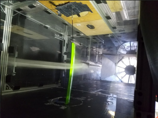
Week 5-Bon Jovi Lyrics Here
Week 5, the halfway point! Only one wind tunnel test this week, the rest was spent in the conference room starting to put together a presentation, and painstakingly stepping through a video frame-by-frame trying to calculate the frequency of vortex shedding on our wing after the flow detaches (preliminary estimates place this number at 40 Hz).
After the Great Wing Bending of April 2018, we decided to fix the wing flexibility problem by performing the ever-elegant solution of shoving a carbon rod in the wing. We figured that placing the carbon rod at about the quarter chord of the wing would allow it to counteract most of the bending the wing experienced. We drilled a hole out of the wing, then tried to stuff the carbon rod in further. All told, we probably managed to get the carbon rod in to a depth of about 4 inches. That should be good enough, right?
That’s still not ideal, and even though the reinforced wing did actually bend less than the original wing, Dr. Doig still likened it to a banana. Such a strong curve definitely affected the angle that we were able to observe stall (it’s safe to say that most airfoils, let alone the 4412, stall well before 22°).
The reason that the wing, reinforced or not, stalled at such a late angle of attack is due to changes in the local angle of attack of the wing. At first I thought the bending would cause such changes, but thinking it over further, I realized that this wouldn’t change the local angle of attack that much. I realized that if anything, the wing must be twisting in a sort of weathervane effect, causing it to have a much lower angle of attack than what is indicated on the winch. This effect must have been stronger on the unreinforced wing, considering we never actually observed stall on that wing.
This twist comes from two likely places: one being that the wing we made didn’t fit in the turntable perfectly, and two that the wing was made of EPP foam, which is a lot less stiff than typical wing materials.
The final thing that we did was attempt to calculate the Strouhal number for the wing once the flow had separated. This necessitated finding the frequency of vortex shedding off the wings. We didn’t actually know how fast the slow-mo was on a Galaxy S8, so some trickery was required: by filming a timer in slow motion, we were able to find out how many seconds passed with each frame, which allowed an fps calculation. (The Galaxy S8 takes slow mo video at 240 frames per second). Then came the meticulous flipping frame by frame through the video to find the exact moment the vortex gets shed off the wing. We found that a similar image showed up every six or so frames, meaning that the vortices were being shed at a pace of about 40 Hz. What does this mean? A little more interpretation is needed on that question.
Today’s fact of the week: did you know a pangram, or a holoalphabetic sentence, is a sentence that uses every letter in the English alphabet? They’re often used to display typefaces, as you can see we did on our slides below:

My favorite pangram is “sphinx of black quartz, judge my vow”, which I think we can all agree is objectively the far cooler way to display an alphabet. There are far more examples, but I think perhaps the most applicable to aerospace engineers is: “ Pack my box with five dozen liquor jugs.”

Source for this adorable image
1 note
·
View note

Video
youtube
Recent changes to the Golden Gate Bridge's guardrails created an otherworldly wail from the bridge. I performed a bit of fluid dynamical detective work to break down what we're hearing. (Video credit: KPIX CBS News; submitted by Christina T.)
285 notes
·
View notes
Photo
Petr Strouhal https://stro90.wixsite.com/petrstrouhal https://www.instagram.com/pe.stro.archive/
1 note
·
View note
Photo
Petr Strouhal
1 note
·
View note
Photo

ILEANA: La Galaxia de Andrómeda, a 700.ooo años luz, que se puede mirar a simple vista en una noche clara, está más cerca que tú. Otros ojos solitarios estarán mirándome desde Andrómeda, en la noche de ellos. Yo a ti no te veo. Ileana: la distancia es tiempo, y el tiempo vuela. A 200 millones de millas por hora el universo se está expandiendo hacia la Nada. Y tú estás lejos de mí como a millones de años.
Ernesto Cardenal
Ph: Frantisek Strouhal
#frantisek strouhal#ph#paper texture#mixedmedia#color printer#ernesto cardenal#poesia#a millones de años#esto es inhumano
12 notes
·
View notes
Text
Vom Wagnis, Seiten zu streifen: Ein Hymnus an die Freiheit des Lesens und die sinnliche Macht des Buches – Ernst Strouhals Essays und Reportagen eröffnen neue Welten im Blättern und Verweilen
Ernst Strouhals Über kurz oder lang: Essays und Reportagen (2024) entfaltet sich als eine wahre Entdeckungsreise durch die Kultur des Lesens, Schreibens und Archivierens. Die Essays zeichnen sich durch eine immense Vielschichtigkeit aus, wobei besonders das Kapitel „Über das Blättern – Verzetteltes Schreiben, zerstreutes Lesen“ hervorsticht. Strouhal, Professor und versierter Kulturpublizist,…
0 notes
Note
Totally hate to be a bother if there is already a post you’ve made about it, but I couldn’t seem to find any in the FAQ. I want to delve into writing historical fiction for Ancient Egypt eventually, as I’ve got an idea for a paranormal-romancey-esque story, and I want to make it as historically accurate as reasonably possible (since the protag is an Egyptologist herself). Do you have any advice for depicting it realistically/researching in particular areas or in any specific books? Thank you! :)
Nah no worries, I haven't answered anything like this specifically yet! So recommendations for historical accuracy and realistic depictions depend on a few things, the first of which is the time period of ancient Egypt your story deals with. I don't know if you've already made decisions about that, but the easiest Dynastic period to set it in would be the New Kingdom, since we have the most material from that time period. Any earlier than that and you have to deal with gaps in our knowledge, as well as a very different kind of Egypt from the image popular media paints (no horses or khepesh swords, for example).
There's a book I like to recommend for research into daily life specifically for fiction writing, which is Life of the Ancient Egyptians by Eugen Strouhal. It has a somewhat too optimistic tendency which borders on romanticising at points, but not in a way that would lead to awkward or harmful representations of the ancient Egyptians. Personally I think it's well-suited as a research work for fiction writers because it places emphasis on the good and human things. When you read it you get a good sense of ancient Egypt as the very verdant, very rich society it was, as opposed to the "dusty barren sand cities" image Hollywood likes to concoct. So in a sense, it takes the kind of liberties I'd like more writers writing about ancient Egypt to take.
Other than that, assuming you're wanting to write New Kingdom (though depending on whether you're writing about elite or non-elite), I'd see if you can pick up Andrea McDowell's Village Life in Ancient Egypt. It deals with the worker's village of Deir el-Medina and life there. Caveat: DeM isn't a "normal" Egyptian village but we do have a ton of information on it, and it isn't necessarily a bad thing to base any fictional villages on this one imo.
From a personal point of view, I can recommend writing about the Middle Kingdom, despite the relative lack of material. Wolfram Grajetzki has some excellent and accessible (some for free) overview works that deal with this period that will give you a solid base. The Egyptian Middle Kingdom, and Middle Kingdom Studies (various authors) are great.
No matter the time period, I'd supplement with Gillian Vogelsang-Eastwood's Pharaonic Egyptian Clothing for the all-important "what are these people even wearing" question. imo, that's a big one in terms of realism. The same goes for Steven Snape's The Complete Cities of Ancient Egypt.
Now, as for the realistic portrayal of an Egyptologist character, my one big tip would be: do. not. infodump.
I know that sounds like just bog standard advice for any genre of book, but in this case there's a second reason to avoid them: having your Egyptologist main character infodump is the way to mark them out as not an actual expert. Not because we never talk about ancient Egypt in real life (we do), but because we don't really talk to ourselves about Egypt in the way of a novel infodump. Absolutely have them explain something super specific to another character, whilst forgetting that the other character doesn't have the full context to understand most of what the fuck they're saying though, that's something we do all the time. Just don't infodump basic concepts, that's half the job done when it comes to realistic portrayals of Egyptologists.
And as always, my evergreen tip: do your research, and then take the liberties your narrative needs to make it the best version of your story (while keeping respect for the ancient Egyptians themselves in mind, but I don't think I need to tell you based on the way you asked this question).
Lastly, I can't technically make any promises considering my health/energy for the foreseeable future, but if there's anything you want me to proofread, feel free to ask!
#egyptology#writing#writing advice#forgot to mention: vogelsang's book is no longer for sale but i have a PDF I can link you!
99 notes
·
View notes
Photo

Petr Strouhal
#Petr Strouhal#InCase#InCase4#InCase.4#heavier than a death in the family#photography#intercession#intercessions gallery
1 note
·
View note
Photo

Connection, photography by KyeongCheol Park for HUF Magazinehttp://hufmagazine.com/connection-photography-by-kyeongcheol-park-for-huf-magazine/
2 notes
·
View notes
Text
Computational Examination of Aerodynamics Forces and Evolution of Vortex Shedding of Flow Past Three Square Cylinders at Two Symmetrical Vee Shapes-Iris Publishers
Authored by Salwa Fezai*

Abstract
The flow past three square cylinders at two symmetrical vee shapes has been investigated by a finite-volume method numerical technique. The two-dimensional computations have been performed for different Reynolds number (Re) ranging from 1 to 180 in order to consider different flow regimes; the steady, the periodic and the turbulent flow. The validation of the code with the available literature results regarded both the reliability of the computed solutions and the overall resulting efficiency of the methods. Velocity profiles, vorticity contours and integral parameters such as Strouhal number, drag and lift coefficients have been presented and analyzed. Steady and unsteady regimes of flow have been observed by monotonously changing the Re value, leading to the prediction of the critical Reynolds number for each configuration considered. Furthermore, the change in the geometry of the obstacle is found to affect dramatically the emergence of the Hopf bifurcation points. The oscillatory periodic wake is also seen to be influenced by the Strouhal number, which varies with obstacle shape and the Re values. Relevant outcomes of this work are the estimation of the vortex shedding frequencies and the prediction of the best configuration considering the computation of the lift and drag coefficients.
Keywords:Staggered square cylinders; Flow regimes; Vortex shedding; Strouhal number; Numerical simulation; Critical Reynolds number; Lift and drag coefficients
Nomenclature
(Nomenclature)
Table 1:
Introduction
The analysis of incompressible fluid flow around bluff bodies has engaged a particular attention of researchers due to its great importance in both aerodynamics and engineering. This type of flow becomes more and more complicated when single bluff body is replaced with multiple bluff bodies in different shapes and arrangements. This complexity in flow causes strong interactions in wakes and considerably modifies the fluctuation of aerodynamic forces. Thus, it is important to understand the dramatic change in aerodynamics characteristics and evolution of vortex shedding frequency in the wake. In fact, many studies show that Reynolds number and the type of square cylinder arrangement has ability to change flow behavior for different flow states. In this vein, we may cite the work of Cheng et al. [1]. They have reported that the vortex shedding and wake development behind the square cylinder are significantly dependent on both the magnitude of the shear rate and the Reynolds number. One can also mention the numerical investigation of Berrone et al. [2]. Their results performed the influence of the Reynolds number on the appearance criteria of different regimes such as crawling scheme, the steady and unsteady with releases of vortices. In addition, Mukhopadhay et al. [3] analyzed the structure of a flow around a square obstacle for different Reynolds number and for different positions of the obstacle. They determined the critical Reynolds number from which the flow becomes periodic and they concluded that the frequency starts at Re = 87 for a blockage ratio B/H = 0.25.
To understand the appearance criteria of steady regime, one can also refer to the investigation of Fezai et al. [4] who analyzed the vortex at different arrangements of the two shapes. Analysis of the flow evolution shows that with increasing Re beyond a certain critical value, the flow becomes unstable and undergoes a bifurcation. The authors demonstrated that the transition to unsteady regime is performed by a Hopf bifurcation and the critical Reynolds number beyond which the flow becomes unsteady is hence determined for each configuration. Lankadasu & Vengadesan [5] observed that the critical Reynolds number is reduced with increasing shear. It was found that the mean drag coefficient decreases either with increasing shear for a particular Reynolds number or with increasing Reynolds number for a particular shear parameter. Sohankar & Etminan [6] investigated the fluid flow around tandem square cylinders in laminar flow regime. Their results showed that the flow was steady when Re≤35 and unsteady periodic when Re≥40. Gera et al. [7] used the Computational Fluid Dynamics (CFD) technique to investigate the 2D steady flow around a square obstacle. The simulation was performed for flow around the square shape end to analyze the wake behavior and Reynolds number was taken from nearly 50 to 250. The coefficient of lift and velocity in the wake region were monitored to calculate the Strouhal number. Bhattacharyya & Maiti [8] numerically analyzed the wake structure behind a square cylinder placed near the lower wall. They found that the wall causes a difference in strength between the two vortex rows and showed that the strength of the positive vortices from the bottom of the cylinder lowers with the decrease of the height between the barrier and the bottom wall. Subsequently, the average drag coefficient weakens with the reduction of the ratio of the standard height. They also proved that the cylinder has a large positive lift when brought close to the wall. The influence of the obstacle orientation has been analyzed by Sajjad & Sohn [9]. They observed that orientation of a square cylinder has a significant effect on the shape and size of the recirculation bubble. They concluded that wake formation and separation processes are asymmetric for angles 22.5 and 30 degrees. In addition, a minimum in drag coefficient and maximum in Strouhal number is observed at a square cylinder orientation of 22.5. The main reason for the minimum drags coefficient at 22.5 is attributed to the wake asymmetry originated from shear layers of unequal lengths on each side of the cylinder. The wake asymmetry increases the transverse velocity, which further increases the base pressure, and hence lowers drag. This factor (wake asymmetry) is counterbalanced by an increase in the projected area. However, it was revealed that the former has an overall stronger influence at small cylinder angles shown by the drag coefficient minimum at an orientation of 22.5. Furthermore, they observed that the separation distance between the alternating vortices depend upon the cylinder orientation. On another hand, it is known in literature that the flow structure around two square cylinders is more complex than that around a single square cylinder. For instance, Burattimi & Agrawal [10] analyzed the flow around two square cylinders at a Reynolds number of 73 and reported different ranges of the wake flow regimes. Abbasi & Islam [11] also simulated wake interactions of a flow around two square cylinders that are placed in line with a fixed space ratio equal to 3.5. They concluded that the unsteady regime appears when the Reynolds number reaches the value 55.
Rao et al. [12] investigated the effect of the space ratio on the flow around two square cylinders arranged side by side. They found that the frequency of vortex shedding is different in two wakes. The upper frequency is smaller than the lower frequency for small rations (s<1.4). However, when the space rations increase, the frequency of vortex shedding is almost equal in two wakes. They analyzed the influence of the space ratio and Reynolds number on the drag and lift force. The difference of time-averaged drag and lift coefficients of the cylinders decreases with the increase in space ratios. When s=2.0 and 2.5, the curves for the time-averaged drag and lift coefficient with different Reynolds numbers are seen to be smooth. The authors also reported that when s=1.5 and 1.8, the curves are smooth under Re<140, but will be fluctuant under Re>140 because of the nonlinear interaction between the wakes and the instability of flow which becomes stronger with the increase in Reynolds numbers. Furthermore, Adeeb et al. [13] investigated computationally the wake flow of two square cylinders by varying the corner radius to understand the effect of the gap spacing’s role and the wake flow pattern at Re = 100. They found that the flow characteristics and vortex shedding depend significantly on the corner radius and gap spacing. They concluded that a square cylinder exhibited the maximum average drag value and an inverse behavior was observed in the case of a circular cylinder. In addition, aerodynamic forces were reduced by rounding the corner radius. The staggered geometry of different square cylinders is much different from tandem and inline configurations because more than one spacing is introduced between the cylinders. In such case the flow characteristics become different from those in the case of single spacing. Compared to tandem and inline arrangement, the staggered arrangement has received very less attention of analysis. Among the authors who analyzed this type of arrangement, one can cite Lee & Yang [14]. The authors investigated the flow around two cylinders for Re ≤ 160. At staggered orientation of 45° and Re =160, they identified four different flow regimes. They reported that gap flow can induce separation on the downstream cylinder which asa result increases the vortex shedding phenomena. Aboueian & Sohankar [15] examined the effect of the gap spacing on the flow over two square cylinders in staggered arrangement at Re=150. By changing the gap spacing between cylinders, five different flow regimes are identified and classified. Islam et al. [16,17] examined the influence of separation rations and Reynolds number for flow around squares cylinders. They found that the flow structure depends on both separation ratio and Reynolds number. The average mean drag coefficient decreases while Strouhal number increases as the gap ratio (g) increases. They observed that as this parameter value increases the average mean drag coefficient and Strouhal number approaches to single rectangular cylinder value.
The flow behind three square cylinders in two different triangular arrangements was investigated numerically by Rahman et al. [18]. They reported that the Strouhal number varied between 0.0132 and 0.2003 in both arrangements. The authors also found that the mean drag coefficient and Strouhal number of all threesquare cylinders approached single square cylinder with the increase in the gap ratio. Yang et al. [19] analyzed numerically the flow pattern and vortex suppression regions for three circular cylinders with two different staggered arrangements. In the first arrangement a primary cylinder was placed in front of downstream two side by side cylinders and in the second arrangement a primary cylinder was placed in the wake of upstream two side by side cylinders. Their results show that in the first arrangement, the vortex shedding behind the primary cylinder was suppressed by the downstream two side by side cylinders at 100≤Re≤200. They also reported that in the second arrangement the vortex shedding of the primary cylinder was suppressed by the upstream two side by side cylinders at 103≤Re≤175. We can also mention the work of Yang et al. [20] who arranged three stationary circular cylinders in such a way that one cylinder was placed in front of two side by side cylinders and investigated the effect of the gap ratio in the range from g=1-10 for Re=200. They observed steady flow region at 1≤g≤1.2 and 2.5 ≤g≤3.1 and unsteady flow region at 1.3≤g≤2.4 and 3.2≤g≤10. They also found regular drag and lift coefficient in steady flow region which became irregular in unsteady flow region. From the previous studies about fluid interaction with solid bodies, it can be observed that there is very limited numerical work available about the flow mode transitions around three staggered square cylinders at low values of Re. The flow around bluff bodies of square cross section is an important fundamental problem of engineering. Also, the staggered square cylinders geometry is vital in the sense that it is very important in practical engineering applications. Therefore, a detailed analysis of flow past three staggered square cylinders is needed. Furthermore, this study will definitely enhance the fluid–structure interaction database. Keeping in view these facts the current numerical study is performed to fully analyze four important features of the flow past three staggered square cylinders in vee shape:
The first task is essentially composed of six parts. Firstly, we present the configuration of the physical problem. The second part is devoted to presentation of equations and boundary conditions. The numerical method used for solving the system of Navier-Stokes equations in its dimensionless form in the case of a two-dimensional (2D) incompressible flow is presented in the third part. The fourth part is dedicated to the validation of the numerical in-house code used and followed finally by results and discussions. The fifth part is devoted to results and discussions. Finally, we will draw conclusions from this study in a final part.
Physical Problem
(Figure 1) The configuration of the current problem is sketched in Figure 1. Two configurations will be considered by varying the arrangement of the three cylinders C1, C2 and C3. For the first configuration the obstacle is composed of three cylinders C1, C2 and C3 as shown in the figure. For the second configuration the arrangement of the three cylinders will be different from the first configuration. In Figure 2 we have schematized the two configurations that will be studied and examined (Figure 2).
Governing flow equations
The physical problem is governed by the Navier–Stokes equations for two-dimensional incompressible fluid flow. The continuity and momentum equations are written in dimensionless form expressed as follows:
In the momentum equation, a dimensionless number appears that is the Reynolds number
expressed by:
Boundary Conditions
The boundary conditions for this physical problem are as following:
1. At the channel entrance:
1. The horizontal u- velocity component has a uniform form u0=1 The vertical component of the velocity v is set to zero.
2. On the obstacle, non-slip conditions are imposed; u = 0 and v = 0
Numerical Method
The dimensionless Navier-Stokes equations were numerically solved utilizing the following numerical technique based on the finite volume method [22]. The temporal discretization of the time derivative is performed by an Euler backward second-order implicit scheme. Nonlinear terms are evaluated explicitly; then, viscous terms are treated implicitly. The strong velocity–pressure coupling present in the continuity and the momentum equations is handled by applying the projection method [23]. A Poisson equation, with the divergence of the intermediate velocity field as the source term, is then computed to obtain the pressure correction and the real velocity field. A finite volume method was utilized on a staggered grid system in order to discretize the system of equations to be solved. Furthermore, the QUICK scheme of Hayase et al. [24] is applied to minimize the numerical diffusion for the advective terms. The discretized equations are computed utilizing the red and black point successive over-relaxation method [25] with the choice of optimum relaxation factors. Besides, the resolution of the Poisson equation is performed by applying an accelerated full multi-grid method [26].
The convergence of the numerical results is established at each time step according to the following criterion:
Where f and t indicates the iteration, time levels. The generic variable f stands for u, v or p. In the above inequality, the subscript sequence (i, j) stands for the grid indexing in the x, and y directions respectively. In conclusion, it is worth noting that computations were performed by applying a developed home code named “NASIM” (Navier Stokes Incompressible Multigrid) [27,28] utilizing finite volume method and the numerical procedure described above.
Results and Discussion
Grid independence test
The construction of the mesh is the first step in any numerical simulation. The used meshes in this investigation are based on a staggered grid where scalar quantities (pressure ...) are located at the center of the cell, while the velocity components are defined at the centers of faces of the volume controls. In order to ensure accuracy, the grids have denser clustering at the vicinity of the barrier where strong gradients are expected. Conversely, away from the obstacle where the expected gradients are low, larger meshes are preferred.
It is worth noting that the grid independence study was conducted for two different non- uniform grids, namely, m*n=560*340 and m*n=768*160. In the current investigation, independence of numerical results from the mesh size was assumed when the difference in the simulated values computed between two consecutive grids was less than 1%. It was concluded from the deviation values obtained that, a non-uniform grid of m*n=768*160 is sufficiently fine to ensure the grid independent solution and provides a good compromise between accuracy and CPU time in the range of variables to be investigated. Hence, the grid m*n=768*160 is applied to perform all subsequent calculations. For better clarification, Figure 3 is schematized describing the mesh used in the present simulations (Figure 3).
Time step independence test
To ensure the accuracy of the results, it is necessary to verify the numerical procedure. The determination of the time step to be utilized in all calculations is very important, since a too large time step size will yield inaccurate results while an excessively smalltime step is computationally inefficient. Furthermore, several time step refinements were performed for the present simulations with non-uniform grid m*n=768*160. To ensure the temporal convergence of results, two Figures 4 & 5 are reported describing the temporal evolution of the lift coefficient and horizontal velocity components, respectively (Figures 4,5).
From Table 1, it is confirmed that the results of the calculations with the time step Δt = 0.001 are nearly identical to the results with Δt = 0.0025 and Δt = 0.0005. That’s why the time step Δt = 0.001 is applied in all simulations (Table 1).
Code validation
To give more confidence to the results of the current simulations, some quantitative and qualitative comparisons with other numerical investigations presented in the literature have been carried out. The physical problem that is used for the validation of the in-house code “NASIM” is the physical model investigated by Breuer et al. [29]. In the current study, validation of the simulations was carried out on a non-uniform mesh of dimension m*n =560*340 as the mesh used by Breuer et al. [29]. The study was conducted over a range of Reynolds number varying from 10 to 180 and analysis of the effect of this parameter on the evolution of the Strouhal number and lift and drag coefficients was carried out. Consequently, the effect of Re on the Strouhal number (Figure 6) was performed. It is noted that for relatively low Reynolds numbers (50 < Re < 130) the Strouhal number increases with Re values. A significant change in the structure of flow takes place, namely the movement of separation point of the trailing edge to the leading edge of the square cylinder. The Strouhal number is at a maximum at nearly Re = 140 then decreases again for higher Reynolds numbers (Figure 6).
The resulting physical parameter like St obtained from these computations is presented in table 2 along with percentage deviation in the code verification with Ref. [29] and Ref. [30]. It is clear from the results that deviation percentage with Ref. [30] is weaker with that of Ref. [29]. Note that the maximum deviation percentage with Ref. [29] and Ref. [30] is respectively 9.69% (when Re = 200) and 2.91% (when Re = 180). In fact, this percentage of maximum deviation has been obtained for the large Reynolds numbers and this leads to the weak refinement of the computing grid. In other words, in order to minimize the error, it is necessary to increase and further refine the mesh for large Reynolds values. In fact, by further incrementing the Reynolds number, more instabilities of the flow may occur, and this may cause the appearance of more vortices and small structures, and for a better visualization of the flow pattern and to capture its structures, the mesh must be further refined (Table 2).
As observed, Figure 5 and Table 2 confirm that our results are in good agreement with the results of Breuer et al. [29] & Galleti et al. [30] and this comparison validates our computer code making confidence on the presented results. It is also worth noting that validation of the computer code has already been presented by Fezai et al. [31,32] which is a contribution of the current investigation.
Analysis of the evolution of vortex shedding of flow
Steady regime
In the previous section, the code validation was discussed. More detailed flow pattern, which is greatly dependent on the geometry of the obstacle, is further investigated in Figure 7 where vorticity contours at Re = 1 relatively to the considered configurations are presented. It is clear that the flow is creeping and the viscous force being preponderant. It can be seen that the fluid remains attached to the obstacle for each configuration and no detachment is observed. Thus, we note the symmetry of the flow with respect to the longitudinal axis. The flow is formed by two almost symmetrical counter-rotating recirculating lobes attached to the obstacle. It is confirmed that the geometry of the obstacle did not modify the structure of the flow since both configurations have the same structure (Figure 7).
The intensity of the viscous force is reduced by augmenting Re to a certain value, during which the separation of the laminar boundary layers occurs. Figure 8 depicts the contours of the iso-vorticities of the two configurations considered for Re=10 and 20. It is observed that the wakes of the two configurations are similar. As displayed in the figure, the state of the flow remains steady. The flow is always symmetrical with respect to the longitudinal axis but loses its symmetry with respect to the upstream and the downstream. A wake appears formed by two symmetrical counter-rotating recirculating lobes attached to the obstacle and occupying the whole volume. Due to the increase of Re, the forces of inertia strengthen and prevent the boundary layer to remain attached to the obstacle and starts to favor a depression in the wake zone. We may note the beginning of birth of the vortex that develops far from the obstacle in the second configuration when Re = 20 because one approaches the bifurcation point towards the unsteady regime (Figure 8).
Hopf Bifurcation point
In this section the hop bifurcation point will be determined and discussed. It can be concluded that the flow is oscillatory from a certain Reynolds value. This periodic behavior occurs when the Reynolds number exceeds the critical value (Rec). It should be noted that the critical value of Re strongly depends on the geometry of the obstacle. Indeed, we consider performing several simulations for several Reynolds for both considered configurations. In order to compute the critical Reynolds number for each configuration, we start from Re = 20 and enhance it with the increment of 0.5 until we find the critical value. From the time when the perturbations change in an oscillatory trend, the flow after the critical point remains periodic in time and undergoes a critical value of Reynolds number. Besides, the square root of the amplitude of the solution increases with the bifurcation parameter. This means that the square of the amplitude of u and v velocity components must be proportional to the value of Re after the bifurcation. It should be noted that the amplitude of the velocity component (u or v) is defined
The values of the constants a and b are determined (see Figure 9) and the values of the critical Reynolds numbers Rec for the two configurations are reported in Table 3 (Figure 9).
The transition to the unsteady regime is found to begin in the second configuration and then in the first configuration. It is clear that the bifurcation points of the steady regime to the unsteady one is very much influenced by the change of the geometry of the obstacle. Therefore, the two configurations considered in this investigation generate a large reduction in the value of the critical Reynolds number. In addition, these obstacles accelerate the birth and generation of vortices. Therefore, we find that the two configurations generate a significant lessening in the critical value of the Reynolds number compared with a square cylinder (Rec=53).
The percentage reduction of Rec for both configurations was determined in Table 4. We determined that the best decline of Rec is seen for the second configuration and the smaller reduction corresponds to the first configuration (Table 3).
Table 2:Influence of time step (Δt) at Re = 50.
Table 3:Comparison of results for the flow past a single square cylinder in terms of percentage reduction.
Table 4:Comparison of results for the flow past a single square cylinder in terms of percentage reduction.
Table 5:Comparison of results for the flow past a single square cylinder in terms of percentage reduction.
Table 6:Mean values of the drag coefficient of both configurations for different Reynolds numbers.
Unsteady regime
As the Reynolds number exceeds the critical value, the flow becomes unsteady. At this stage, the instabilities are triggered which generates a noticeable change in the flow structure. To better analyze this change, Figure 10 is presented illustrating the effect of the Reynolds number on the iso-vorticities of the two configurations. For low Reynolds numbers (Re = 40 and 60), it is noted that the structure of the flow is similar in both configurations. A pair of vortices appears with opposing signs alternately separating behind each obstacle. In fact, the influence of the viscous force becomes negligible. However, the intensity of the inertial force strengthens with Reynolds increase so this force becomes dominant knowing that this number is defined as the ratio of the inertia force by the viscous force. As the Reynolds number augments, the shape and size of the vortices change in both configurations. This change is due to the influence of the obstacle geometry on the vortex structure. Therefore, we note that in the first configuration the shape of the vortices of negative sign becomes very elongated and these swirls dominate the wake, but the vortices of positive sign keep the round shape. Due to the lengthening of the negative sign vortices, the lateral and longitudinal spacing increases in the wake so this spacing causes a significant change in the fluctuation of the pressure. On the other hand, in the second configuration, the shape of the vortices of negative sign remains round but a significant change establishes in the shape of the vortices of positive sign which makes these vortices very elongated. The intensity of these positive vortices dominates and increases while increasing the Reynolds number. It can also be seen that the interaction between vortices of different intensities leads to a vortex structure proportional to the shape of the obstacle with a lateral and longitudinal spacing as proportional to the geometry of the obstacle.
It is clear that the flow pattern depends strongly on the shape of the obstacle. It can be deduced then that the two configurations generate a significant change in the characteristics of the wake be cause the lengthening of these vortices causes a remarkable spacing in the wake. Therefore, the spacing in the wake leads to diminishing the pressure and enhancing the speed. In order to verify the fluctuation of the velocity in the wake of both configurations, the variation of the horizontal component (u) of the velocity as a function of the Reynolds number is shown in Figure11. It can be seen that the velocity variation in both configurations increases monotonically as a function of the Reynolds number. However, it should be noted that the variation of the speed is very high in the second configuration and the smallest fluctuation of (u) is noted in the first configuration. It can be deduced that the second configuration causes a sharp decrease in the variation of the pressure compared with the first configuration (Figures 10,11).
Analysis of the fluctuation of Strouhal number
In this study, a fast Fourier transform of the time series for the lift coefficients is used to determine the Strouhal number. It can be seen in Figure 12 that the Strouhal number of the two configurations increases monotonously with Rewhen30 ≤ Re ≤ 80. This depends on the inertial force which strengthens with the increase of Re. When 30 ≤ Re ≤ 80, it is noted that the values of the frequency of detachment of the vortices are very close in both configurations. It is clear that the obstacles geometry has no effect on the evolution of the Strouhal number when the Reynolds number slightly varies. Moreover, we find that the first configurations reach the maximum before the second configuration. For the first configuration, this maximum is in the vicinity of a Reynolds which is equal to 90. On the other hand, for the second configuration, this maximum value was noted for a Reynolds number very close to 100 (Figure 12).
When Re ≥ 90, a considerable change in the fluctuation of the Strouhal number in both configurations is observed and at this stage appears the effect of the geometry and the symmetry of the configurations on the fluctuation of the Strouhal number. The values of St in the second configuration become greater than the values of St in the first configuration. This change can be due to the influence of the geometry of the obstacle on the detachment of the vortices. The first configuration hence generates a reduction in the fluctuation of St compared with the second one, and this reduction becomes very important for higher values of the Reynolds number.
Figure 13 illustrates a comparison between the values of St of both configurations with the case of a square cylinder. It is observed that the two configurations generate a significant reduction in the values of the Strouhal number compared with the square cylinder case. It is clear that this reduction becomes more significant with Re and seems to be very important when the Reynolds number has a value 160. The percentage of reduction of St for both configurations was determined in Table 4. We find that for low Reynolds numbers (Re = 60 and 80) the best reduction is caused by the second configuration and the lowest reduction corresponds to the first one. Starting from the value Re=100, the percentage of reduction augments in the first configuration and becomes the highest in this configuration compared to the other one. Note that the maximum reduction percentage in the first arrangement and the second one is respectively 29.10% (when Re = 140) and 27.90% (when Re = 160) (Table 4).
Analysis of the fluctuation of the average drag coefficient
The drag coefficient corresponds to the force applied to the body in the flow direction which is made dimensionless by the density of the fluid. Its velocity at upstream direction (U∞ ) is a characteristic surface calculated from the side of the shape and its size.
The drag coefficient is computed as follows:
The subscripts f, r, b and t refer to the front, rear, bottom and top surfaces of the obstacle.
The average values of the drag coefficient of the two configurations when Re varies from 1 to 180 are reported in Table 5 (Table 5).
Table 5 shows that the average drag coefficient (CD) of the two configurations has a fairly high value at Re = 1 since the velocity seems to be much weakened and hence a higher pressure is established. Thus, we may predict the higher value of CD in the first configuration and the lowest one in the second configuration. It can then be concluded that the first configuration generates a pressure rise when compared with the second one. When the Reynolds number is further raised, a sharp decrease is noticed in the fluctuation of the average drag coefficient and observed for both configurations. This decrease is related to the growth of the intensity of the forces of inertia and the lowering of the intensity of the viscous ones. In addition, it can be seen that when the flow remains steady (Re = 1-10-20), the highest values of CD are noted in the first configuration and the lowest values are obtained for the second configuration. The diminution in CD can be explained by the velocity strengthening as shown in Figure 12 and therefore the decrease in pressure because the change in pressure is inversely proportional to the speed variation. By further enhancing the Reynolds number, a decrease in the CD values is seen and this leads to lessening pressure and strengthening the speed (Figure 11). It should be noted that from a Re = 30 the CD values are very close in both configurations. Consequently, the influence of the geometry of the obstacle on the variation of the drag force strengthens and becomes significant while lowering the Reynolds number. However, the effect of the geometry decreases while increasing the Reynolds number. In the range 60 ≤ Re ≤ 180, the flow undergoes an unsteady behavior. The highest CD values are then noted in the second configuration. This is due to the enhancement in the intensity of the forces applied by the flow on this obstacle and to the decrease in pressure which becomes almost negligible. Conversely at steady state where the pressure forces are very high and the velocity variation is very low, CD values become very low in the first configuration when the flow state is unsteady.
Figure 14 is plotted in order to compare the values of the average drag coefficient of the two configurations considered in this study with the CD values of a square cylinder. It can be seen that the shape of the two configurations considerably modifies the variation of pressure and velocity in the flow. This results in a change in the fluctuation of the drag force. Therefore, it can be observed that the CD values noted in the flow around a square cylinder are very small compared to the values of the two configurations. It can be deduced then that the two configurations generate an enhancement in the intensity of the drag force compared to the case of a square cylinder.
Analysis of the fluctuation of the average lift coefficient
The subscripts f, r, b and t refer to the front, rear, bottom and top surfaces of the shape.
To understand the link between the fluctuation of the lift force and the shape of the obstacle, we present the figure 15. This figure shows the variation of the time average value of the lift coefficient versus the Reynolds number for both configurations. First, it is noted that the largest value of CL corresponds to the first configuration and the lowest value is related to the second one. As the Reynolds number augments, the curve relative to the second configuration exhibits a rising trend. By cons, in the first configuration the average value of the lift coefficient lowers. It is clear that the curves of the two configurations evolve symmetrically with respect to the curve of the square configuration. This indicates that the direction of the lift force applied to the first configuration is opposite to the direction of the lift force of the second configuration. Therefore, this reversal evolution in the direction of the lift force is due to the shape of both configurations. When 10 ≤ Re ≤ 180, the average lift coefficients of the first configuration are negative, while those of the second configuration are positive. It can be seen then that the geometry of the obstacle considerably affects the fluctuation of the lift force. Indeed, it can be observed that the first configuration generates a large reduction in the average lift coefficient compared with the square configuration. However, the second configuration generates a considerable enhancement in the values of the average lift coefficient (Figure 15).
Conclusion
The flow patterns past three square cylinders at two symmetrical vee shapes have been numerically performed for 1 ≤ Re ≤ 180. Two different arrangements were considered and compared in terms of flow behavior and characteristics. An accelerated multigrid implicit volume method was used as a numerical technique for the present study. Firstly, the computations were carried out for flow behind a single square cylinder in order to check the validity and accuracy of the in-house NASIM code. Then, the flow characteristics of both considered arrangements were investigated in terms of vorticity contour visualization, time evolutions analysis of drag and lift coefficients. Main findings are summarized below:
1. It is found that both the arrangements and the geometry of the obstacle affect the flow characteristics significantly as well as the appearance of bifurcation point from steady to the unsteady state. Indeed, it is seen that the transition to the unsteady state begins in the second configuration from (Rec = 22.37) and then emerge in the first configuration precisely at the value (Rec = 22.45). Besides, both configurations considered in this study generate an important decline in the critical Reynolds number value and accelerate the birth and vortices generation.
2. Influence of the obstacle geometry on the vortex detachment and the Strouhal number variation versus Re have been analyzed and discussed for the two configurations. It is seen that varying the arrangements leads to a considerable modification in the fluctuation of the Strouhal number.
3. In addition, fluid behavior of both arrangements were analyzed and compared with single cylinder case. The numerical results show that the two configurations generate a significant reduction in the values of the Strouhal number compared with the square cylinder. This reduction reinforces with increment in Re and becomes more significant when the Reynolds number reaches the value 160.
4. When analyzing the effect of the obstacle geometry on the flow structure and the frequency of vortices detachment, the results also suggest that both arrangements considerably modify the variation of pressure and velocity in the flow. This results in a variation in the typical fluctuations of the drag force.
5. Considering the geometry influence of both configurations on the lift, it is observed that the geometry of the obstacle noticeably affects the fluctuation of the lift force with symmetrical evolutions for both configurations. This reversal distribution trend demonstrates that the direction of the lift force applied to the first configuration is opposite to the lift force direction of the second one due to the shape of both of them.
Read More...FullText
For more article in Current Trends in Civil & Structural Engineering (CTCSE) Please click on https://irispublishers.com/ctcse/
Indexing List of Iris Publishers: https://medium.com/@irispublishers/what-is-the-indexing-list-of-iris-publishers-4ace353e4eee
Iris publishers google scholar citation: https://scholar.google.co.in/scholar?hl=en&as_sdt=0%2C5&q=irispublishers&btnG=
2 notes
·
View notes