#multiclass classification in machine learning
Explore tagged Tumblr posts
Text
The Ultimate Guide to Finding the Best Datasets for Machine Learning Projects

Introductions:
Datasets for Machine Learning Projects, high-quality datasets are crucial for the development, training, and evaluation of models. Regardless of whether one is a novice or a seasoned data scientist, access to well-organized datasets is vital for creating precise and dependable machine-learning models. This detailed guide examines a variety of datasets across multiple fields, highlighting their sources, applications, and the necessary preparations for machine learning initiatives.
Significance of Quality Datasets in Machine Learning
The performance of a machine learning model can be greatly influenced by the dataset utilized. Factors such as the quality, size, and diversity of the dataset play a critical role in determining how effectively a model can generalize to new, unseen data. The following are essential criteria that contribute to dataset quality:
Relevance: The dataset must correspond to the specific problem being addressed.
Completeness: The presence of missing values should be minimal, and all critical features should be included.
Diversity: A dataset should encompass a range of examples to enhance the model's ability to generalize.
Accuracy: Properly labeled data is essential for effective training and assessment.
Size: Generally, larger datasets facilitate improved generalization, although they also demand greater computational resources.
Categories of Datasets for Machine Learning
Machine learning datasets can be classified based on their structure and intended use. The most prevalent categories include:
Structured vs. Unstructured Datasets
Structured Data: This type is organized in formats such as tables, spreadsheets, or databases, featuring clearly defined relationships (e.g., numerical, categorical, or time-series data).
Unstructured Data: This encompasses formats such as images, videos, audio, and free-text data.
Supervised vs. Unsupervised Datasets
Supervised Learning Datasets: These datasets consist of labeled examples where the target variable is known (e.g., tasks involving classification and regression).
Unsupervised Learning Datasets: These do not contain labeled target variables and are often employed for purposes such as clustering, anomaly detection, and dimensionality reduction.
Domain-Specific Datasets
Healthcare: Medical imaging, patient records, and diagnostic data.
Finance: Stock prices, credit risk assessment, and fraud detection.
Natural Language Processing (NLP): Text data for sentiment analysis, translation, and chatbot training.
Computer Vision: Image recognition, object detection, and facial recognition datasets.
Autonomous Vehicles: Sensor data, LiDAR, and road traffic information.
Numerous online repositories offer open-access datasets suitable for machine learning applications. Below are some well-known sources:
UCI Machine Learning Repository
The UCI Machine Learning Repository hosts a wide array of datasets frequently utilized in academic research and practical implementations.
Noteworthy datasets comprise:
Iris Dataset (Multiclass Classification)
Wine Quality Dataset
Banknote Authentication Dataset
Google Dataset Search
Google Dataset Search facilitates the discovery of datasets available on the internet, consolidating information from public sources, governmental bodies, and research institutions.
AWS Open Data Registry
Amazon offers a registry of open datasets available on AWS, encompassing areas such as geospatial data, climate studies, and healthcare.
Image and Video Datasets
COCO (Common Objects in Context): COCO Dataset
ImageNet: ImageNet
Labeled Faces in the Wild (LFW): LFW Dataset
Natural Language Processing Datasets
Sentiment140 (Twitter Sentiment Analysis)
SQuAD (Stanford Question Answering Dataset)
20 Newsgroups Text Classification
Preparing Datasets for Machine Learning Projects

Prior to the training of a machine learning model, it is essential to conduct data preprocessing. The following are the primary steps involved:
Data Cleaning
Managing missing values (through imputation, removal, or interpolation)
Eliminating duplicate entries
Resolving inconsistencies within the data
Data Transformation
Normalization and standardization processes
Feature scaling techniques
Encoding of categorical variables
Data Augmentation (Applicable to Image and Text Data)
Techniques such as image flipping, rotation, and color adjustments
Utilizing synonym replacement and text paraphrasing for natural language processing tasks.
Notable Machine Learning Initiatives and Their Associated Datasets
Image Classification (Utilizing ImageNet)
Objective: Train a deep learning model to categorize images into distinct classes.
Sentiment Analysis (Employing Sentiment140)
Objective: Evaluate the sentiment of tweets and classify them as either positive or negative.
Fraud Detection (Leveraging Credit Card Fraud Dataset)
Objective: Construct a model to identify fraudulent transactions.
Predicting Real Estate Prices (Using Boston Housing Dataset)
Objective: Create a regression model to estimate property prices based on various attributes.
Chatbot Creation (Utilizing SQuAD Dataset)
Objective: Train a natural language processing model for question-answering tasks.
Conclusion
Selecting the appropriate dataset is essential for the success of any machine learning endeavor. Whether addressing challenges in computer vision, natural language processing, or structured data analysis, the careful selection and preparation of datasets are vital. By utilizing publicly available datasets and implementing effective preprocessing methods, one can develop precise and efficient machine learning models applicable to real-world scenarios.
For those seeking high-quality datasets specifically designed for various AI applications, consider exploring platforms such as Globose Technology Solutions for advanced datasets and AI solutions.
0 notes
Text
EECS 498-007 / 598-005 Deep Learning for Computer Vision Assignment 2 solved
In this assignment, you will implement various image classification models, based on the SVM / Softmax / Two-layer Neural Network. The goals of this assignment are as follows: Implement and apply a Multiclass Support Vector Machine (SVM) classifier Implement and apply a Softmax classifier Implement and apply a Two-layer Neural Network classifier Understand the differences and tradeoffs between…
0 notes
Text
EECS 498-007 / 598-005 Deep Learning for Computer Vision Assignment 2
In this assignment, you will implement various image classification models, based on the SVM / Softmax / Two-layer Neural Network. The goals of this assignment are as follows: Implement and apply a Multiclass Support Vector Machine (SVM) classifier Implement and apply a Softmax classifier Implement and apply a Two-layer Neural Network classifier Understand the differences and tradeoffs between…
0 notes
Text
EECS 498-007 / 598-005 Deep Learning for Computer Vision Assignment 2 solution
In this assignment, you will implement various image classification models, based on the SVM / Softmax / Two-layer Neural Network. The goals of this assignment are as follows: Implement and apply a Multiclass Support Vector Machine (SVM) classifier Implement and apply a Softmax classifier Implement and apply a Two-layer Neural Network classifier Understand the differences and tradeoffs between…
0 notes
Text
Mastering Machine Learning Basics: Intermediate Course for Beginners Explained
Are you intrigued by the fascinating world of machine learning but find yourself stuck between beginner and advanced levels? Fear not! In this comprehensive guide, we'll delve into the essentials of an intermediate machine learning course designed specifically for beginners. Whether you're a student, a professional looking to upskill, or simply curious about this revolutionary field, this article aims to demystify complex concepts and pave the way for your mastery of machine learning basics.
Understanding the Prerequisites
Before diving into an intermediate course, it's crucial to have a solid understanding of the foundational concepts of machine learning. Familiarize yourself with programming languages such as Python and essential libraries like NumPy, Pandas, and Scikit-learn. Additionally, grasp the basics of statistics and linear algebra, as they form the backbone of many machine learning algorithms.
Exploring Intermediate Topics
Regression Analysis:
In this section, you'll learn about regression models, which are used to predict continuous outcomes. Dive into techniques such as linear regression, polynomial regression, and ridge regression, understanding how to interpret coefficients and assess model performance.
Classification Algorithms:
Move beyond binary classification and explore multiclass classification algorithms like logistic regression, decision trees, and support vector machines (SVM). Understand the importance of feature selection, hyperparameter tuning, and evaluating classification models using metrics like accuracy, precision, and recall.
Dimensionality Reduction:
Delve into dimensionality reduction techniques such as principal component analysis (PCA) and t-distributed stochastic neighbor embedding (t-SNE). Learn how to reduce the number of features in your dataset while preserving essential information, thereby improving model efficiency and interpretability.
Clustering Methods:
Discover unsupervised learning techniques like K-means clustering and hierarchical clustering. Understand how these algorithms group similar data points together without predefined labels, enabling insights into underlying patterns and structures within your data.
Ensemble Learning:
Explore the power of ensemble methods such as bagging, boosting, and random forests. Learn how combining multiple models can lead to better predictive performance and increased robustness, making your machine learning models more resilient to noise and overfitting.
Neural Networks and Deep Learning:
Take your understanding of neural networks to the next level by exploring deep learning architectures like convolutional neural networks (CNNs) and recurrent neural networks (RNNs). Learn about different layers, activation functions, and optimization techniques crucial for building and training sophisticated models.
Natural Language Processing (NLP):
Venture into the realm of NLP, where you'll discover techniques for processing and analyzing human language data. From text preprocessing and tokenization to sentiment analysis and named entity recognition, unlock the potential of machine learning in understanding and generating human language.
Time Series Analysis:
Dive into time series data and learn how to model and forecast sequential data points. Explore techniques such as autoregressive integrated moving average (ARIMA), seasonal decomposition, and recurrent neural networks for capturing temporal patterns and making accurate predictions.
Model Deployment and Interpretability:
Finally, grasp the essential aspects of deploying machine learning models into production environments. Understand the importance of model interpretability, fairness, and ethics, ensuring that your solutions are transparent, accountable, and accessible to all stakeholders.
Hands-on Learning Approach
Throughout the course, emphasize a hands-on learning approach by working on real-world projects and datasets. Leverage online platforms, tutorials, and interactive coding environments to practice implementing algorithms, fine-tuning parameters, and analyzing results. Collaborate with peers, participate in forums, and seek mentorship to accelerate your learning journey and gain valuable insights from experienced practitioners.
Conclusion
Embarking on an intermediate machine learning course for beginners is an exciting journey that opens doors to endless possibilities in the realm of artificial intelligence and data science. By mastering the topics outlined in this guide, you'll develop the skills and confidence to tackle complex problems, build predictive models, and contribute meaningfully to the advancement of technology. Remember, persistence, curiosity, and a willingness to learn are your greatest allies on this exhilarating path towards machine learning mastery. So, roll up your sleeves, sharpen your mind, and embark on this transformative learning experience today!
0 notes
Text
Logistic Regression (Multiclass Classification)

Multiclass Classification using Logistic Regression for Handwritten Digit Recognition
In the realm of machine learning, logistic regression isn't just limited to binary classification tasks. In this tutorial, we'll delve into how logistic regression can be employed for multiclass classification. We'll use the `LogisticRegression` class from the `sklearn` library to predict handwritten digits. To make this journey informative and engaging, we'll illustrate every step with code examples and visualizations.
Loading the Dataset
Before we start building our classifier, let's get acquainted with the dataset we'll be working with. We'll use the `load_digits` function from `sklearn.datasets` to load a collection of 8x8 pixel images of handwritten digits.
from sklearn.datasets import load_digits
import matplotlib.pyplot as plt
digits = load_digits()
# Display the first five images
plt.gray()
for i in range(5):
plt.matshow(digits.images[i])
plt.show()
Dataset Details
The loaded dataset contains the following attributes:
- `DESCR`: Description of the dataset
- `data`: Array of feature vectors representing the digits
- `images`: Images of the handwritten digits
- `target`: Target labels corresponding to the digits
- `target_names`: Names of the target classes (digits 0-9)
Training the Classifier
We'll employ logistic regression to train a multiclass classification model. Let's start by splitting our dataset into training and testing sets using the `train_test_split` function.
from sklearn.linear_model import LogisticRegression
from sklearn.model_selection import train_test_split
# Split the data into training and testing sets
X_train, X_test, y_train, y_test = train_test_split(digits.data, digits.target, test_size=0.2)
# Create and train the logistic regression model
model = LogisticRegression()
model.fit(X_train, y_train)
Evaluating Model Accuracy
Once our model is trained, it's crucial to evaluate its performance. We can do this by calculating the accuracy on the testing set.
accuracy = model.score(X_test, y_test)
print("Model Accuracy:", accuracy)
Making Predictions
We're now equipped to make predictions using our trained model. Let's predict the first five digits from our dataset and observe the results.
predictions = model.predict(digits.data[0:5])
print("Predictions for the first five digits:", predictions)
Visualizing the Confusion Matrix
A confusion matrix provides deeper insights into the performance of our classifier. It reveals how well the model is classifying each digit.
from sklearn.metrics import confusion_matrix
import seaborn as sns
# Predict on the test set
y_predicted = model.predict(X_test)
# Create the confusion matrix
cm = confusion_matrix(y_test, y_predicted)
# Visualize the confusion matrix
plt.figure(figsize=(10, 7))
sns.heatmap(cm, annot=True)
plt.xlabel('Predicted')
plt.ylabel('True')
plt.show()
Conclusion
In this tutorial, we explored how to use logistic regression for multiclass classification. We employed the `LogisticRegression` class from `sklearn` to build a model capable of recognizing handwritten digits. We split the data, trained the model, evaluated its accuracy, made predictions, and visualized the confusion matrix to assess the model's performance. Logistic regression, once thought of as solely binary, showcases its versatility and effectiveness in tackling multiclass classification tasks.
Remember, the journey of machine learning is full of exploration and experimentation. By understanding the techniques and methods available, you'll be better equipped to create intelligent systems that can interpret and classify diverse data.
@talentserve
0 notes
Link
Science and technology have significantly helped the human race to overcome most of its problems. From making people fly in the air to helping them in managing traffic on roads, science has been present everywhere.
#binary classification in machine learning#multiclass classification in machine learning#binary classification in supervised machine learning#classification in machine learning#machine learning algorithm#multilabel classification#multi-class classification#difference between binary and multi-class classification#binary classification vs multiclass classification#binary vs multiclass classification
0 notes
Text
Machine Learning by Andrew Ng week 4 ( Summary )
https://www.coursera.org/learn/machine-learning/lecture/gFpiW/multiclass-classificationhttps://www.coursera.org/learn/machine-learning/lecture/OAOhO/non-linear-hypotheses
Non-linear Hypotheses
https://www.coursera.org/learn/machine-learning/lecture/ka3jK/model-representation-i
neural networks Model Representation I
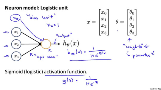
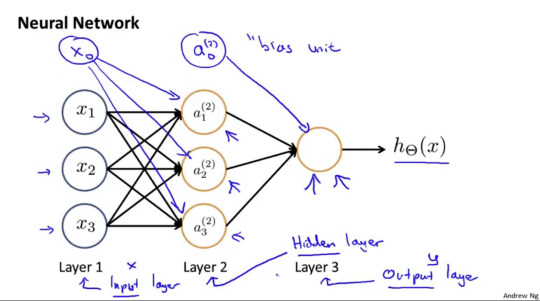
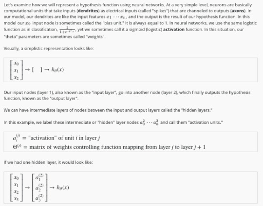
3층구조로 되어있다. 첫번째는 input layer, 두번째는 hidden layer, 마지막은 output layer가 된다.
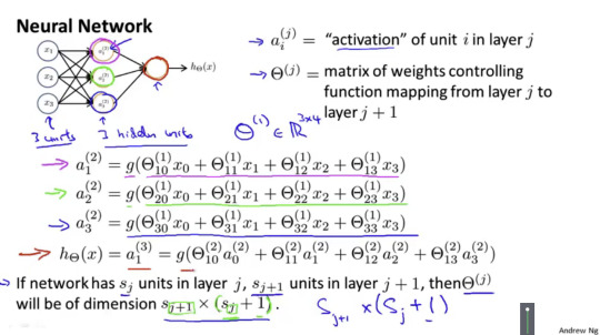
우측 상단 내용은 superscript는 몇번째 layer인지를 알려준다. subscript는 몇번째 unit인지 알려준다는 이야기이다.
그림 하단의 내용은 현layer의 unit 수 * (전단계unit수+1) 의 dimension의 matrix가 된다는 이야기이다.
https://www.coursera.org/learn/machine-learning/supplement/Bln5m/model-representation-i
Model Representation I
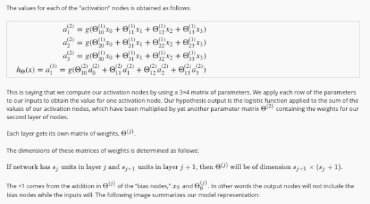
https://www.coursera.org/learn/machine-learning/lecture/Hw3VK/model-representation-ii
neural networks Model Representation II
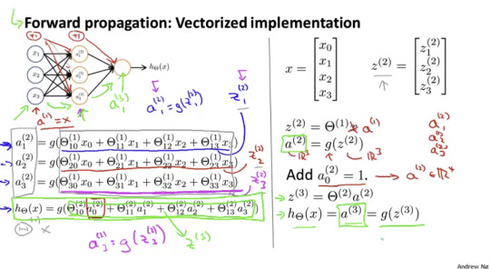
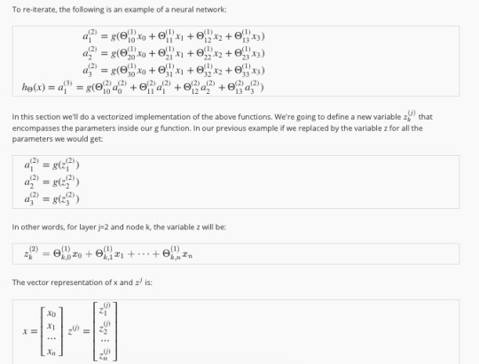
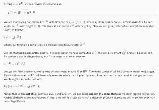
위의 그림은 복잡한 수식을 좀 정리해서 보여준다.
a의 경우는 g(z()) 이라고 축약해서 보여준다. 즉 features x값과 쎄타값을 곱한 결과를 g()에 넣어 계산해서 나온 결과를 a 2라고 한다. 다시 이 a 2를 쎄타2와 곱한다. 곱해서 얻을 결과를 g()에 넣어 나온결과를 a 3라고 한다. 위의 그림에서 a 3는 최종결과이며 h쎄타() 이다.
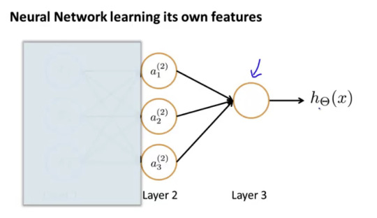
neural networks 에서 마지막 부분만을 잘라서 본다면 이는 logistic regression 과 동일하다, 위의 그림 참조
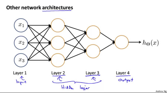
여러겹의 hidden layer가 추가된 예시를 보여준다.
https://www.coursera.org/learn/machine-learning/supplement/YlEVx/model-representation-ii
neural networks Model Representation II
https://www.coursera.org/learn/machine-learning/lecture/rBZmG/examples-and-intuitions-i
neural networks Examples and Intuitions I
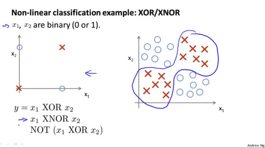
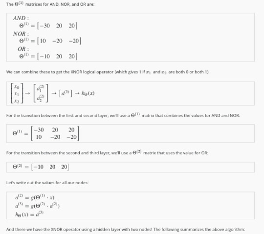
인공신경망으로 xor 논리 연산을 구현 하는 방법
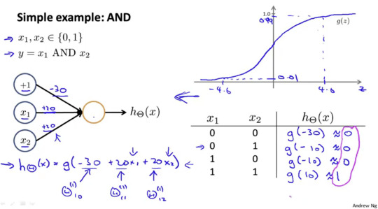
g() 는 sigmoid funciton이고 공식은 아래와 같다
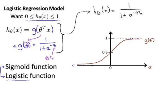
e -4 거듭 제곱의 값은 0.01832 이고 1/1+0.01832 은 0.99 이다. 결론적으로 z 가 4인 경우 0.99 가 된다는 의미이다. 위위그림의 4.0를 기준점으로 정한이유.
or 논리연산을 인공신경망으로 구현한 예시는 아래와 같다.
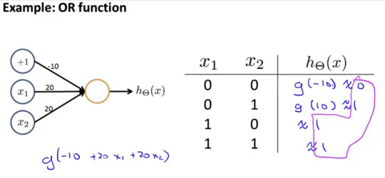
https://www.coursera.org/learn/machine-learning/supplement/kivO9/examples-and-intuitions-i
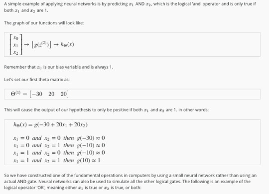
neural networks Examples and Intuitions I
https://www.coursera.org/learn/machine-learning/lecture/solUx/examples-and-intuitions-ii
neural networks Examples and Intuitions II
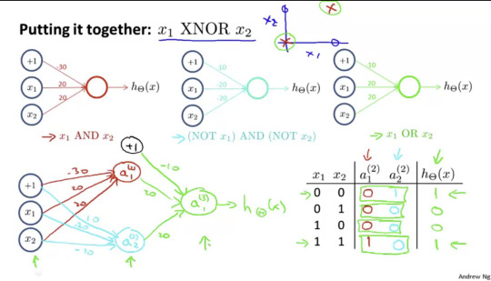
위 그림은 이미 공부한 두개의 unit을 하나로 합쳐서 좀더 복잡한 논리 연산을 구현한 것을 보여준다.
https://www.coursera.org/learn/machine-learning/supplement/5iqtV/examples-and-intuitions-ii
neural networks Examples and Intuitions II
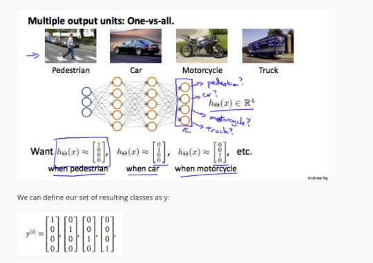
https://www.coursera.org/learn/machine-learning/lecture/gFpiW/multiclass-classification
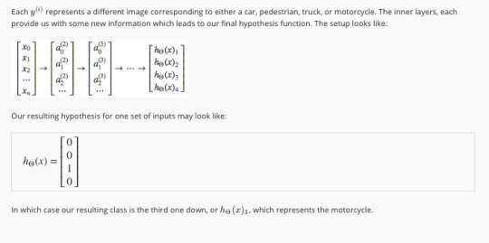
Multiclass Classification
https://www.coursera.org/learn/machine-learning/supplement/xSUml/multiclass-classification
Multiclass Classification
#machine learning#ml#machine#learning#summary#andrew#andrew ng#Multiclass Classification#classification#Neural Networks#Neural#logic#logical#or#and#xor
0 notes
Text
Important libraries for data science and Machine learning.
Python has more than 137,000 libraries which is help in various ways.In the data age where data is looks like the oil or electricity .In coming days companies are requires more skilled full data scientist , Machine Learning engineer, deep learning engineer, to avail insights by processing massive data sets.
Python libraries for different data science task:
Python Libraries for Data Collection
Beautiful Soup
Scrapy
Selenium
Python Libraries for Data Cleaning and Manipulation
Pandas
PyOD
NumPy
Spacy
Python Libraries for Data Visualization
Matplotlib
Seaborn
Bokeh
Python Libraries for Modeling
Scikit-learn
TensorFlow
PyTorch
Python Libraries for Model Interpretability
Lime
H2O
Python Libraries for Audio Processing
Librosa
Madmom
pyAudioAnalysis
Python Libraries for Image Processing
OpenCV-Python
Scikit-image
Pillow
Python Libraries for Database
Psycopg
SQLAlchemy
Python Libraries for Deployment
Flask
Django
Best Framework for Machine Learning:
1. Tensorflow :
If you are working or interested about Machine Learning, then you might have heard about this famous Open Source library known as Tensorflow. It was developed at Google by Brain Team. Almost all Google’s Applications use Tensorflow for Machine Learning. If you are using Google photos or Google voice search then indirectly you are using the models built using Tensorflow.
Tensorflow is just a computational framework for expressing algorithms involving large number of Tensor operations, since Neural networks can be expressed as computational graphs they can be implemented using Tensorflow as a series of operations on Tensors. Tensors are N-dimensional matrices which represents our Data.
2. Keras :
Keras is one of the coolest Machine learning library. If you are a beginner in Machine Learning then I suggest you to use Keras. It provides a easier way to express Neural networks. It also provides some of the utilities for processing datasets, compiling models, evaluating results, visualization of graphs and many more.
Keras internally uses either Tensorflow or Theano as backend. Some other pouplar neural network frameworks like CNTK can also be used. If you are using Tensorflow as backend then you can refer to the Tensorflow architecture diagram shown in Tensorflow section of this article. Keras is slow when compared to other libraries because it constructs a computational graph using the backend infrastructure and then uses it to perform operations. Keras models are portable (HDF5 models) and Keras provides many preprocessed datasets and pretrained models like Inception, SqueezeNet, Mnist, VGG, ResNet etc
3.Theano :
Theano is a computational framework for computing multidimensional arrays. Theano is similar to Tensorflow , but Theano is not as efficient as Tensorflow because of it’s inability to suit into production environments. Theano can be used on a prallel or distributed environments just like Tensorflow.
4.APACHE SPARK:
Spark is an open source cluster-computing framework originally developed at Berkeley’s lab and was initially released on 26th of May 2014, It is majorly written in Scala, Java, Python and R. though produced in Berkery’s lab at University of California it was later donated to Apache Software Foundation.
Spark core is basically the foundation for this project, This is complicated too, but instead of worrying about Numpy arrays it lets you work with its own Spark RDD data structures, which anyone in knowledge with big data would understand its uses. As a user, we could also work with Spark SQL data frames. With all these features it creates dense and sparks feature label vectors for you thus carrying away much complexity to feed to ML algorithms.
5. CAFFE:
Caffe is an open source framework under a BSD license. CAFFE(Convolutional Architecture for Fast Feature Embedding) is a deep learning tool which was developed by UC Berkeley, this framework is mainly written in CPP. It supports many different types of architectures for deep learning focusing mainly on image classification and segmentation. It supports almost all major schemes and is fully connected neural network designs, it offers GPU as well as CPU based acceleration as well like TensorFlow.
CAFFE is mainly used in the academic research projects and to design startups Prototypes. Even Yahoo has integrated caffe with Apache Spark to create CaffeOnSpark, another great deep learning framework.
6.PyTorch.
Torch is also a machine learning open source library, a proper scientific computing framework. Its makers brag it as easiest ML framework, though its complexity is relatively simple which comes from its scripting language interface from Lua programming language interface. There are just numbers(no int, short or double) in it which are not categorized further like in any other language. So its ease many operations and functions. Torch is used by Facebook AI Research Group, IBM, Yandex and the Idiap Research Institute, it has recently extended its use for Android and iOS.
7.Scikit-learn
Scikit-Learn is a very powerful free to use Python library for ML that is widely used in Building models. It is founded and built on foundations of many other libraries namely SciPy, Numpy and matplotlib, it is also one of the most efficient tool for statistical modeling techniques namely classification, regression, clustering.
Scikit-Learn comes with features like supervised & unsupervised learning algorithms and even cross-validation. Scikit-learn is largely written in Python, with some core algorithms written in Cython to achieve performance. Support vector machines are implemented by a Cython wrapper around LIBSVM.
Below is a list of frameworks for machine learning engineers:
Apache Singa is a general distributed deep learning platform for training big deep learning models over large datasets. It is designed with an intuitive programming model based on the layer abstraction. A variety of popular deep learning models are supported, namely feed-forward models including convolutional neural networks (CNN), energy models like restricted Boltzmann machine (RBM), and recurrent neural networks (RNN). Many built-in layers are provided for users.
Amazon Machine Learning is a service that makes it easy for developers of all skill levels to use machine learning technology. Amazon Machine Learning provides visualization tools and wizards that guide you through the process of creating machine learning (ML) models without having to learn complex ML algorithms and technology. It connects to data stored in Amazon S3, Redshift, or RDS, and can run binary classification, multiclass categorization, or regression on said data to create a model.
Azure ML Studio allows Microsoft Azure users to create and train models, then turn them into APIs that can be consumed by other services. Users get up to 10GB of storage per account for model data, although you can also connect your own Azure storage to the service for larger models. A wide range of algorithms are available, courtesy of both Microsoft and third parties. You don’t even need an account to try out the service; you can log in anonymously and use Azure ML Studio for up to eight hours.
Caffe is a deep learning framework made with expression, speed, and modularity in mind. It is developed by the Berkeley Vision and Learning Center (BVLC) and by community contributors. Yangqing Jia created the project during his PhD at UC Berkeley. Caffe is released under the BSD 2-Clause license. Models and optimization are defined by configuration without hard-coding & user can switch between CPU and GPU. Speed makes Caffe perfect for research experiments and industry deployment. Caffe can process over 60M images per day with a single NVIDIA K40 GPU.
H2O makes it possible for anyone to easily apply math and predictive analytics to solve today’s most challenging business problems. It intelligently combines unique features not currently found in other machine learning platforms including: Best of Breed Open Source Technology, Easy-to-use WebUI and Familiar Interfaces, Data Agnostic Support for all Common Database and File Types. With H2O, you can work with your existing languages and tools. Further, you can extend the platform seamlessly into your Hadoop environments.
Massive Online Analysis (MOA) is the most popular open source framework for data stream mining, with a very active growing community. It includes a collection of machine learning algorithms (classification, regression, clustering, outlier detection, concept drift detection and recommender systems) and tools for evaluation. Related to the WEKA project, MOA is also written in Java, while scaling to more demanding problems.
MLlib (Spark) is Apache Spark’s machine learning library. Its goal is to make practical machine learning scalable and easy. It consists of common learning algorithms and utilities, including classification, regression, clustering, collaborative filtering, dimensionality reduction, as well as lower-level optimization primitives and higher-level pipeline APIs.
mlpack, a C++-based machine learning library originally rolled out in 2011 and designed for “scalability, speed, and ease-of-use,” according to the library’s creators. Implementing mlpack can be done through a cache of command-line executables for quick-and-dirty, “black box” operations, or with a C++ API for more sophisticated work. Mlpack provides these algorithms as simple command-line programs and C++ classes which can then be integrated into larger-scale machine learning solutions.
Pattern is a web mining module for the Python programming language. It has tools for data mining (Google, Twitter and Wikipedia API, a web crawler, a HTML DOM parser), natural language processing (part-of-speech taggers, n-gram search, sentiment analysis, WordNet), machine learning (vector space model, clustering, SVM), network analysis and visualization.
Scikit-Learn leverages Python’s breadth by building on top of several existing Python packages — NumPy, SciPy, and matplotlib — for math and science work. The resulting libraries can be used either for interactive “workbench” applications or be embedded into other software and reused. The kit is available under a BSD license, so it’s fully open and reusable. Scikit-learn includes tools for many of the standard machine-learning tasks (such as clustering, classification, regression, etc.). And since scikit-learn is developed by a large community of developers and machine-learning experts, promising new techniques tend to be included in fairly short order.
Shogun is among the oldest, most venerable of machine learning libraries, Shogun was created in 1999 and written in C++, but isn’t limited to working in C++. Thanks to the SWIG library, Shogun can be used transparently in such languages and environments: as Java, Python, C#, Ruby, R, Lua, Octave, and Matlab. Shogun is designed for unified large-scale learning for a broad range of feature types and learning settings, like classification, regression, or explorative data analysis.
TensorFlow is an open source software library for numerical computation using data flow graphs. TensorFlow implements what are called data flow graphs, where batches of data (“tensors”) can be processed by a series of algorithms described by a graph. The movements of the data through the system are called “flows” — hence, the name. Graphs can be assembled with C++ or Python and can be processed on CPUs or GPUs.
Theano is a Python library that lets you to define, optimize, and evaluate mathematical expressions, especially ones with multi-dimensional arrays (numpy.ndarray). Using Theano it is possible to attain speeds rivaling hand-crafted C implementations for problems involving large amounts of data. It was written at the LISA lab to support rapid development of efficient machine learning algorithms. Theano is named after the Greek mathematician, who may have been Pythagoras’ wife. Theano is released under a BSD license.
Torch is a scientific computing framework with wide support for machine learning algorithms that puts GPUs first. It is easy to use and efficient, thanks to an easy and fast scripting language, LuaJIT, and an underlying C/CUDA implementation. The goal of Torch is to have maximum flexibility and speed in building your scientific algorithms while making the process extremely simple. Torch comes with a large ecosystem of community-driven packages in machine learning, computer vision, signal processing, parallel processing, image, video, audio and networking among others, and builds on top of the Lua community.
Veles is a distributed platform for deep-learning applications, and it’s written in C++, although it uses Python to perform automation and coordination between nodes. Datasets can be analyzed and automatically normalized before being fed to the cluster, and a REST API allows the trained model to be used in production immediately. It focuses on performance and flexibility. It has little hard-coded entities and enables training of all the widely recognized topologies, such as fully connected nets, convolutional nets, recurent nets etc.
1 note
·
View note
Text
[ad_1] Learning artificial intelligence (AI) is becoming increasingly important for both technical and non-technical professionals, as it has the potential to revolutionize various industries and provide innovative solutions to complex problems. With free AI courses and online certifications, individuals can acquire the necessary knowledge and skills to stay relevant in today’s rapidly evolving job market.The Machine Learning Specialization by DeepLearning.AI and Stanford OnlineThe Machine Learning Specialization by DeepLearning.AI and Stanford Online is a foundational online program that provides a broad introduction to modern machine learning. This three-course specialization is taught by Andrew Ng, an AI visionary who has led critical research at Stanford University and groundbreaking work at Google Brain, Baidu, and Landing.AI to advance the AI field.Other notable instructors include Eddy Shyu, curriculum product manager at DeepLearning.AI; Aarti Bagul, a curriculum engineer; and Geoff Ladwig, another top instructor at DeepLearning.AI.The first course in the specialization is “Supervised Machine Learning: Regression and Classification,” which covers building machine learning models in Python using popular machine learning libraries NumPy and scikit-learn, and building and training supervised machine learning models for prediction and binary classification tasks, including linear regression and logistic regression.The second course is “Advanced Learning Algorithms,” which teaches building and training a neural network with TensorFlow to perform multiclass classification, applying best practices for machine learning development so that your models generalize to data and tasks in the real world, and building and using decision trees and tree ensemble methods, including random forests and boosted trees.The third and final course is “Unsupervised Learning, Recommenders, Reinforcement Learning,” which covers using unsupervised learning techniques for unsupervised learning, including clustering and anomaly detection, building recommender systems with a collaborative filtering approach and a content-based deep learning method, and building a deep reinforcement learning model.By the end of this specialization, one will have mastered key concepts and gained practical know-how to quickly and powerfully apply machine learning to challenging real-world problems. If you’re looking to break into AI or build a career in machine learning, the Machine Learning Specialization is a great place to start.CS50’s Introduction to Artificial Intelligence with Python by Harvard UniversityCS50’s Introduction to Artificial Intelligence with Python, offered by Harvard University, is an introductory course exploring modern artificial intelligence concepts and algorithms. The course is free on edX, but students can purchase a verified certificate for an additional fee. The instructors for the course are Gordon McKay, professor of the practice of computer science at Harvard University; Brian Yu, senior preceptor in computer science at Harvard University; and David Malan. Students will dive into the ideas that give rise to technologies like game-playing engines, handwriting recognition and machine translation. This course teaches students how to incorporate machine learning concepts and algorithms into Python programs through a series of hands-on projects.Related: A brief history of artificial intelligenceStudents will gain exposure to the theory behind graph search algorithms, classification, optimization, reinforcement learning, and other topics in artificial intelligence and machine learning. By the end of the course, students will have experience in libraries for machine learning, and knowledge of artificial intelligence principles that will enable them to design intelligent systems of their own.AI For Everyone by Coursera in collaboration with DeepLearning.AIAI for Everyone is an online course offered by Coursera in collaboration with DeepLearning.
AI. This course is designed for non-technical learners who want to understand AI concepts and their practical applications. It provides an overview of AI and its impact on the world, covering the key concepts of machine learning, deep learning and neural networks.The course is taught by Andrew Ng, a renowned AI expert and founder of DeepLearning.AI. He is also a co-founder of Coursera and has previously taught popular online courses on machine learning, neural networks and deep learning. The course consists of four modules, each covering a different aspect of AI. These are:What is AI?Building AI projectsBuilding AI in your companyAI and societyThe course is self-paced and takes approximately 10 hours to complete. It includes video lectures, quizzes and case studies that allow students to apply the concepts they have learned using popular programming languages such as Python.The course is free to audit on Coursera, and financial aid is available for those who cannot afford the fee. A certificate of completion is also available for a fee.Machine Learning Crash Course with TensorFlow APIs by GoogleThe Machine Learning Crash Course with TensorFlow APIs is a free online course offered by Google. It’s designed for beginners who want to learn about machine learning and how to use TensorFlow, which is a popular open-source library for building and deploying machine learning models.The course covers the following topics:Introduction to machine learning and TensorFlowLinear regressionClassificationNeural networksRegularizationTraining and validationConvolutional neural networksNatural language processingSequence modelsThroughout the course, you’ll learn about different machine-learning techniques, and how to use TensorFlow application programming interfaces (APIs) to build and train models. The course also includes hands-on exercises and coding assignments, which will help you gain practical experience building and deploying machine learning models.The course is available for free on Google’s website, and is self-paced so that you can learn at your own speed. Upon completion, you’ll receive a certificate of completion from Google.Related: 5 emerging trends in deep learning and artificial intelligenceIntroduction to AI by IntelThe Intel® AI Fundamentals Course is an introductory-level course that teaches the fundamentals of artificial intelligence and its applications. It covers topics such as machine learning, deep learning, computer vision, natural language processing and more. The free and self-paced course includes modules that can be completed in any order. The eight-week program includes lectures and exercises. Each week, students are expected to spend 90 minutes completing the coursework. The exercises are implemented in Python, so prior knowledge of the language is recommended, but students can also learn it along the way. The course does not offer a certificate of completion, but students can earn badges for completing each module. The course is designed for software developers, data scientists and others interested in learning about AI.Ready to join the AI revolution?By taking advantage of the above resources, individuals can become part of the growing AI industry and contribute to shaping its future. Additionally, the ChatGPT Prompt Engineering for Developers course, developed in collaboration with OpenAI, offers developers the opportunity to learn how to use large language models (LLMs) to build powerful applications in a cost-effective and efficient manner. The course is taught by two renowned experts in the field of AI: Isa Fulford and Andrew Ng. Whether a learner is a beginner or an advanced machine learning engineer, this course will provide the latest understanding of prompt engineering and best practices for using prompts for the latest LLM models. With hands-on experience, one will learn how to use LLM APIs for various tasks, including summarizing, inferring, transforming text and expanding, and building a custom chatbot.
This course is free for a limited time, so don’t miss out on the opportunity to join the AI revolution. [ad_2] Source
0 notes
Text
An Introduction to Deep Learning
Deep Learning is at the cutting edge of what machines can do, and developers and magnate definitely need to comprehend what it is and how it works. This special kind of algorithm has far gone beyond any previous benchmarks for category of images, text, and voice. Are you interest in learning "Deep Learning" you can follow best Coursera deep learning courses for more information It also powers some of the most intriguing applications worldwide, like autonomous lorries and real-time translation. There was definitely a bunch of excitement around Google's Deep Learning based AlphaGo beating the very best Go gamer in the world, however business applications for this innovation are more immediate and potentially more impactful. This post will break down where Deep Learning fits into the environment, how it works, and why it matters.
What is Deep Learning?
To understand what deep learning is, we first need to comprehend the relationship deep learning has with machine learning, neural networks, and artificial intelligence. The very best way to consider this relationship is to imagine them as concentric circles: Deep learning is a specific subset of Machine Learning, which is a particular subset of Artificial Intelligence. For private meanings: Artificial Intelligence is the broad required of developing machines that can think intelligently Machine Learning is one method of doing that, by utilizing algorithms to glean insights from data (see our mild introduction here). Deep Learning is one way of doing that, using a specific algorithm called a Neural Network. Do not get lost in the taxonomy-- Deep Learning is simply a type of algorithm that appears to work truly well for forecasting things. Deep Learning and Neural Nets, for most purposes, are efficiently synonymous. If individuals try to puzzle you and argue about technical meanings, do not stress over it: like Neural Nets, labels can have numerous layers of significance. Neural networks are influenced by the structure of the cerebral cortex. At the fundamental level is the perceptron, the mathematical representation of a biological nerve cell. Like in the cortex, there can be numerous layers of interconnected perceptrons. Input values, or to put it simply our underlying data, get travelled through this "network" of covert layers till they eventually assemble to the output layer. The output layer is our prediction: it may be one node if the design simply outputs a number, or a couple of nodes if it's a multiclass classification issue. The covert layers of a Neural Net perform modifications on the data to ultimately feel out what its relationship with the target variable is. Each node has a weight, and it multiplies its input worth by that weight. Do that over a couple of different layers, and the Web is able to essentially control the data into something significant. To figure out what these small weights need to be, we usually use an algorithm called Backpropagation. The great reveal about Neural Nets (and a lot of Machine Learning algorithms, really) is that they aren't all that wise-- they're basically simply feeling around, through trial and error, to attempt and discover the relationships in your data. In his popular Coursera course on Machine Learning, Teacher Andrew Ng uses the analogy of a lazy hiker to describe how most algorithms end up working: "we position a fictional hiker at various points with simply one instruction: Walk only downhill up until you can't walk down anymore.". The hiker doesn't actually understand where she's going-- she simply feels around to discover a course that might take her down the mountain. Our algorithm is the very same-- it's probing to figure out how to make the most precise predictions. The last worths that each our our nodes in a Neural Web takes on is a reflection of that procedure. In the 1980s, a lot of neural networks were a single layer due to the cost of calculation and accessibility of data. Nowadays we can afford to have more covert layers in our Neural Nets, hence the name "Deep" Learning. The various types of Neural Networks available for usage have actually also proliferated. Designs like Convolutional Neural Webs, Reoccurring Neural Internet, and Long Short-Term Memory are discovering compelling usage cases across the board.
1 note
·
View note
Text
MOT: a Multi-Omics Transformer for multiclass classification tumour types predictions
Motivation Breakthroughs in high-throughput technologies and machine learning methods have enabled the shift towards multi-omics modelling as the preferred means to understand the mechanisms underlying biological processes. Machine learning enables and improves complex disease prognosis in clinical settings. However, most multi-omic studies primarily use transcriptomics and epigenomics due to their over-representation in databases and their early technical maturity compared to others omics. For complex phenotypes and mechanisms, not leveraging all the omics despite their varying degree of availability can lead to a failure to understand the underlying biological mechanisms and leads to less robust classifications and predictions. Results We proposed MOT (Multi-Omic Transformer), a deep learning based model using the transformer architecture, that discriminates complex phenotypes (herein cancer types) based on five omics data types: transcriptomics (mRNA and miRNA), epigenomics (DNA methylation), copy number variations (CNVs), and proteomics. This model achieves an F1-score of $98.37%$ among 33 tumour types on a test set without missing omics views and an F1-score of $96.74%$ on a test set with missing omics views. It also identifies the required omic type for the best prediction for each phenotype and therefore could guide clinical decision-making when acquiring data to confirm a diagnostic. The newly introduced model can integrate and analyze five or more omics data types even with missing omics views and can also identify the essential omics data for the tumour multiclass classification tasks. It confirms the importance of each omic view. Combined, omics views allow a better differentiation rate between most cancer diseases. Our study emphasized the importance of multi-omic data to obtain a better multiclass cancer classification. Availability and implementation: MOT source code is available at url{https://github.com/dizam92/multiomic_predictions}. http://dlvr.it/ScthNX
0 notes
Text
Why Do We Need NLP?
Why Do We Need NLP? Natural language processing (NLP) is the process of analyzing words and phrases to determine their meaning. However, this process is far from perfect. Some of the challenges include semantic analysis, which is not easy for programs to grasp. The abstract nature of language can also be difficult for programs to process. Furthermore, a sentence can have multiple meanings depending on the speaker's inflection or stress. Another challenge is that NLP algorithms might not pick up subtle changes in voice tone. NLTK The NLTK is a framework that reduces the amount of infrastructure required for advanced projects. NLTK provides predefined interfaces and data structures, which help users create new modules with minimal effort. This way, they can concentrate on the more difficult problems and not on the underlying infrastructure. NLTK is open-source, which means that anyone can contribute to it. To get started with NLTK, you need Python installed. Then, you should install the python compiler and All NLP packages. When this is done, you should open a dialogue box and select "Tokenize text." Tokenization is the process of breaking text into words, sentences, and characters. Two types of tokenizing are used in NLP: nominalization and lexical tokenization. SpaCy SpaCy is a Python package that tokenizes text, processes it into a Doc object, and then returns a result. Its processing pipeline is composed of several components: a lemmatizer, tagger, parser, and entity recognizer. Each component returns a processed Doc. You can learn more about each of these components in the usage guide. SpaCy allows you to create a processing pipeline that includes machine learning components. The first component is a tokenizer, which acts on text to generate a result. From there, you can add a parser or a statistical model. You can also use custom components. Another component is POS tagging. This algorithm tags words with the appropriate part of speech, and changes with context. In this way, spaCy can predict which words are more likely to appear in a given text. Naive Bayes Algorithm The Naive Bayes algorithm is a fast machine learning algorithm that can classify data into binary and multi-class categories. This algorithm is useful in many practical applications. There are several ways to apply Naive Bayes, including regularization and small-sample correction. One of the most popular Naive Bayes variants is the Multinomial Naive Bayes, which is typically used with multivariate, Bernoulli distributions. This version of the Naive Bayes algorithm is fast and extensible, and can classify binary and multiclass data. This algorithm is also computationally cheap. In contrast, it would take a lot of time to build a classifier from scratch. Naive Bayes classifiers take the average of a number of features and assign them to different classes. This makes them ideal for text classification. Masked Language Model A Masked Language Model (MLM) is a machine learning technique that predicts the masked token in a given sentence based on other words in the sentence. Its bidirectional nature allows it to learn from words on both sides of a masked word. The model is often trained with a specific learning objective. It can be applied in many NLP tasks. In particular, it can be applied to speech recognition, question answering, and search. It can be trained using a fraction of the input text and combines that information to make a more accurate representation. This technology is highly computationally efficient and is expected to improve performance on NLP tasks. A Masked Language Model works by taking an entire sentence as input and masking about fifteen percent of words. The model can then predict the words that are left unmasked. It can also learn to represent sentences in a bidirectional manner. It can even learn to predict words from two masked sentences by concatenating them. Conversational AI Conversational AI is an emerging field in computer science. It is a branch of artificial intelligence that uses natural language processing (NLP) to recognize and understand conversations. Until now, conversational AI was limited to speech recognition in the internet. However, with advances in AI and machine learning, conversational AI can now be used in a number of real-world applications. The use of conversational AI in customer service is becoming more widespread. This technology can power intelligent virtual agents that can offer assistance and resolve customer issues. It is already entering the mainstream, and 79% of contact center leaders plan to invest in greater AI capabilities in the next two years. Read the full article
0 notes
Text
What you'll learn Create a Machine Learning app with C#Use TensorFlow or ONNX model with dotnet appUsing Machine Learning model in ASP dotnetUse AutoML to generate ML dotnet modelNote: This course is designed with ML.Net 1.5.0-preview2Machine Learning is learning from experience and making predictions based on its experience.In Machine Learning, we need to create a pipeline, and pass training data based on that Machine will learn how to react on data.ML.NET gives you the ability to add machine learning to .NET applications.We are going to use C# throughout this series, but F# also supported by ML.Net.ML.Net officially publicly announced in Build 2019.It is a free, open-source, and cross-platform.It is available on both the dotnet core as well as the dotnet framework.The course outline includes:Introduction to Machine Learning. And understood how it’s different from Deep Learning and Artificial Intelligence.Learn what is ML.Net and understood the structure of ML.Net SDK.Create a first model for Regression. And perform a prediction on it.Evaluate model and cross-validate with data.Load data from various sources like file, database, and binary.Filter out data from the data view.Export created the model and load saved model for performing further operations.Learn about binary classification and use it for creating a model with different trainers.Perform sentimental analysis on text data to determine user’s intention is positive or negative.Use the Multiclass classification for prediction.Use the TensorFlow model for computer vision to determine which object represent by images.Then we will see examples of using other trainers like Anomaly Detection, Ranking, Forecasting, Clustering, and Recommendation.Perform Transformation on data related to Text, Conversion, Categorical, TimeSeries, etc.Then see how we can perform AutoML using ModelBuilder UI and CLI.Learn what is ONNX, and how we can create and use ONNX models.Then see how we can use models to perform predictions from ASP.Net Core.Who this course is for:This is for newbies who want to learn Machine LearningDeveloper who knows C# and want to use those skills for Machine Learning tooA person who wants to create a Machine Learning model with C#Developer who want to create Machine Learning
0 notes
Text
Homework 02: Discrimination by Regression solution
Homework 02: Discrimination by Regression solution
ENGR 421 / DASC 521: Introduction to Machine Learning In this homework, you will implement a discrimination by regression algorithm for multiclass classification in Matlab, Python, or R. Here are the steps you need to follow: 1. Read Section 10.7.3 (4th edition) or Section 10.8 (3rd edition) from the textbook. 2. You are given a multivariate classification data set, which contains 195…

View On WordPress
0 notes
Text
Machine Learning Homework 3 Solution
Machine Learning Homework 3 Solution
1 SVM vs. Neural Networks In this section, I did experiments on the SVM and MLP using following two datasets: Table 1: Datasets Dataset Classes Size Features breast-cancer 2 683 10 dna 3 3186 180 I tried both binary and multiclass classification tasks on the two classifiers. The size and features of the two datasets is different. Thus, we can compare the performance of SVM and MLP in…

View On WordPress
0 notes