#if they could give me the raw data i could even program something to crawl that offline | Explore Tumblr posts and blogs

kprciffdw · 4 years ago

Text

Ratchet and Kim Possible: The Solanian Revolution-Part 20

They arrived at Qwark's Hideout. After they landed, they gave themselves a little bit a time to look out at the entire place. Kim: "Wow…this is…such a secluded place." Ron: "Yeah, this would seem like a good place to set up a secret hideout but did it have to be someplace so cold?" Kim: "That would make it even more difficult to seek him out." Ron: "Good point." Ratchet: "Come on, guys. Qwark has to be here somewhere."

They rushed out. As they ran through the area, they came across a few nasty, robotic hazards, such as some little pests that they did not think they would ever have to face. Computer voice: "Lawn Ninja Defense System Activated!" Ron: "Oh, no, not the Lawn Ninjas!" Kim: "Heh, so not the drama."

They fought through the little robotic pests and wrecked every single one of them without even a scratch, except for Ron. One of the Lawn Ninjas sliced his pants up almost completely. Ron: "Aw, man! Come on! Seriously?" Ratchet: "I was wondering when that would happen again." Clank: "I thought you guys managed to fix that problem." Kim: "So did I."

Thankfully, the Pants Regenerator was still functioning, so it repaired Ron's pants in a flash. Ratchet: "Well…at least Wade's Pants Regenerator is still working…come on, let's keep going before something else rips up his pants."

They continued on. Ron ran a little slower than the others. Ron: "Right behind you guys."

As they persisted through the area, they found themselves faced by a lot of Qwark bots. Not only did they look like him, but they talked like him, too. Kim: "You've got to be kidding me! Qwark bots?" Ratchet: "Hey, at least we know this is where Qwark set up his base if we didn't know that already." Ron: "Man, it's like a Qwark-infested nightmare!" Kim: "Heh, couldn't have said it better myself, Ron."

They kept going, fighting through many of the Qwark bots as well as several more Lawn Ninjas. They soon hit a roadblock in which they had to rely on Clank and the monkey to help them overcome. After the time extended effort, they were able to overcome the impasse and find Qwark. When they managed to reach him, he was wearing crimson long johns that also went over his head like his hero outfit. He was also wearing his gloves and shoes. He noticed his monkey almost immediately. Qwark: "Hey, little buddy! How did you find me?"

He soon noticed the group a little afterwards. Qwark: "Huh? Oh, it's you guys. What are you doing here?" Kim: "We were looking for you." Ratchet: "We found your secret Holo-vid, Qwark. That's how we were able to find this place." Qwark: "Oh…that…well, I didn't expect you guys to understand." Kim: "Understand what exactly?" Qwark: "You probably think, I would give anything to have a body like that, for one drop of his raw animal magnetism, an iota of…" Ron: "Uh, is he serious right now?" Kim: "I can't tell whether to say yes or no." Ratchet: "OK, enough! We don't want to hear any more of you mindless babbling!" Qwark: "Er…right, let's see, where was I…"

As he continued on and on, Ratchet, Kim and Ron exchanged displeased looks with each other. Qwark: "Ah, yes. But despite my outward appearance of utter perfection, well…um…" Ratchet: "Deep down, you're a cowardly wuss?" Kim: "That pretty much hits the nail on the head." Ron: "Agreed." Qwark: "Uh…no…not…exactly…when I escaped from that star cruiser, cheating death by mere nanoseconds, I suddenly realized something very important: I could have died! Me! Captain Qwark! Imagine an entire galaxy with no more…me." Kim: "Well, one galaxy fell into chaos because of you, so…an entire galaxy without you would have one less strife-inducing nut case." Ratchet: "Good one, Kim." Qwark: "And all of it for what cause? So a few trillion people get turned into robots? Who am I to say who should or should not be turned into a robot? Pffft! Whatever!"

The entire group was appalled by Qwark's apathetic attitude. Ratchet: "You know what? You're pathetic, Qwark! I can't believe I once looked up to you. Come on, guys, let's get out of here."

Ratchet walked out. Ron: "He used to look up to you? That's even more shocking than someone who looks up to me!"

Ron walked out after Ratchet. Qwark: "Uh…I…was it…something I said?" Kim: "Gee, I don't know, everything you've said and done so far clearly demonstrates that you're a bona fide hero." Qwark: "Really?" Kim: "No, of course not. I was being sarcastic, Captain Bozo. Maybe if you started actually being a real hero instead of just acting like one, maybe you would actually start getting some respect for a change."

Kim walked out. Clank was about to walk out, too, but then stopped and looked up at Qwark. Clank: "She is right. The people of this galaxy need you, Qwark. They believe in you. You can give them hope. You have a chance to redeem yourself and become the hero you have always wanted to be."

Clank walked out. The monkey screeched at him once before walking out with the group. Despondent, he looked towards his hero suit.

The group arrived back at their ship. As soon as they got back in, they immediately received a transmission from Sasha. Sasha: "Ratchet! Kim! Where have you been?" Kim: "Sasha!" Ratchet: "Uh…we were just…" Sasha: "Nevermind! The Phoenix is under attack! The shields are…"

The transmission was interrupted for a brief moment. Ratchet: "Sasha!"

The transmission reconnected. Sasha: "To 40%. Life supports are…I think they're getting…aboard the ship. Whatever's on that disk has Nefarious worried…do anything to get it back…Hey, hotshot, if I don't see you again, I just want to tell you…"

The transmission was cut off and did not reconnect again. Kim: "Sorry, Ratchet…I'm afraid…the signal was lost…" Ratchet: "Kim, engage the gravimetric warp drive! Let's get back to the Phoenix as fast as possible!" Kim: "Sure thing, Ratchet!"

They took off and left for the Phoenix.

After returning, they saw that the entire place was under red alert. They also found some of Nefarious' bots throughout the place. Kim: "Whoa…Nefarious has really hit this place hard." Ratchet: "Come on, we have to make sure Sasha and the other crew members are alright."

They rushed out. Ron, however, became easily side-tracked. Ron: "Oh, no! The VG-9000 and virtual menu! I have to make sure they're both OK!"

Ron ran towards their quarters but Kim grabbed him by his shirt collar and pulled him the other way.

They rushed towards the bridge but found that the access transporter was broken. Ron: "Oh, no! They broke the transporter to the bridge!" Kim: "We'll have to find another way to reach the bridge!" Ratchet: "Then, let's get going! We can't stand here and do nothing!"

They hurried along through the newly opened area where they found a crawl space to enter. There, they fought off more robots as they proceeded through. This was where Kim and Ratchet had to really work together. They fought their way through some vicious robots to until eventually, they made it to the bridge.

As soon as they entered, they found Sasha, Helga and Al hiding below the walkway to the captain's seat. Helga: "Well, you certainly took your sweet time." Ratchet: "Hey, it's good to see you, too."

The group walked towards them. Kim: "Is everyone OK?" Sasha: "We're fine, Kim. You guys made it just in time." Ratchet: "Any luck with the data disk?" Al: "Hmph! "Luck" he says." Ron: "So…that's a no?" Al: "No!? Do you think I would be incapable of solving this thing? Hilarious!" Sasha: "Al cracked the encryption. The disc contains a complete copy of Nefarious' battle plan." Kim: "Whoa…Nefarious had every right to be worried." Ron: "Oh, boy, you can say that again." Sasha: "He's going to attack planet after planet, leaving nothing but robots in his wake." Kim: "Well, that seemed pretty obvious." Sasha: "There's more to it. The Biobliterator is so well protected, Nefarious doesn't believe there is any chance we can stop it." Kim: "Oh, I'm sure we'll find a way." Ratchet: "Can we really?" Al: "I estimate our odds at approximately 1 in 63 million, give or take." Kim: "Is that all? I've handled worse." Ratchet: "I don't know, Kim. This may be too much, even for you." Kim: "Even if that is true, there has to be a way to stop it. I won't give up so easily, even if the odds are far beyond anything we can handle." Al: "Um, perhaps there is something. The Biobliterator is programmed to recharge its power cells after each attack." Kim: "Well, there you go. We've got ourselves a potential weakness." Ron: "So, does it have a specific place where it recharges its batteries, or does it have several scattered charge stations?" Sasha: "It's currently recharging at a base on Planet Koros." Kim: "Then that's where we need to go."

They were about to walk out. Ratchet: "By the way, did a little girl and her blue dog stop by here recently?" Sasha: "Um, yeah, they did actually. They gave us a few devices they said would make us immune to the Biobliterator. She said she and her friends are delivering them to everyone in the galaxy, but I don't think they'll be able to deliver them to everyone in time and for some, it's already too late." Ratchet: "Then we have no time to lose. We need to leave now." Sasha: "You guys should hurry because…the next target…is Veldin."

Ratchet, shocked to hear this, growled in anger. Kim: "We'll see to it that attack won't happen." Ratchet: "You said it, Kim."

They rushed out of the bridge and returned to the ship as fast as they possibly could. They then left the Phoenix.

#Kim Possible #Ratchet and Kim Possible Chronicles #Ratchet and Clank #Up Your Arsenal #Starship Phoenix #Ratchet #Clank #Ron Stoppable #Skrunch the monkey #Captain Qwark #Captain Sasha #Helga #Solana Galaxy

1 note · View note

caffeinated-yearning · 5 years ago

Text

The Start of Something Awful

@werewolfpine said I should post my writing and I’m doing it because I will literally never post unless someone forces me to, here’s a snippet of the lore of How Doc Ock Comes To Be, featuring my/Ock’s actual mind thought mannerisms. Technically this has only my S/I Oliver and Doctor Octavius a little at the front end, because I do my best work when it’s one character who thinks too much.

Word Count: ~1.4k Warnings: Self-harm (minor), queasiness (minor), astonishingly sarcastic narrator voice

“Hoshino.”

Oliver looks up from the box; as much as people focused on biorobotics, he rather preferred the metal things he’d been working on. None of that confusion of the ‘bio’ aspect. Cold techne and cold metal, a perfect compliment to his frozen heart. Looked up at his teacher- professor, Otto Octavius, and said nothing.

“The test results..?”

Of course! How could he possibly forget the mind-crippling endeavor of writing up a lab report for the sake of his dear professor? It would never pass off as science if he didn’t suffer the hideous toil of turning his experiment into a report; let it be known that the gods themselves would forbid anyone to simply look at the raw data and draw their own conclusions- no, he has to bring their attention to that all himself.

Ability to self-replicate- [Y] Hive mind program- [Y] Formation of simple and complex shapes- [Y] Link to human minds- concept phase. Mobile complex shapes- concept only. Modify macro chemicals within human body- tested in organic slurry, dubious results. Anything else that could be interesting- hasn’t been conceptualized yet.

“Would you call it a success?”

“If it teaches something new, it is a success.”

“Then have you been taught anything?”

Oh, doctor, do not pretend! This is all just a reinvention of the wheel at this point. Smaller and still programmable they may be, but these are all things that have been done before. They were done decades ago, before everyone found biological machinery to hold more promise. What then is there to learn? Humans disagree with metal, that has been the lesson. Oliver answers in so dry a tone; “discussion section: page three. Sir.”

“So I read.” Oliver returns his attention to his robots, still attentive to the good doctor’s words; “you sound irritated- both in the paper and at present.”

It is proper to smile and shake his head, to set the doctor’s concerns to rest. He fails this task, and in the same dry tone; “I’m not. I have concerns that this research is dated at best.”

“Then you are-.”

Interrupting, and how uncharacteristic that was- “I don’t have the time to be emotional, in any event.” The professor seemed off-put by that. Indeed, it was rude of Oliver to interrupt; he makes note of that, and fails to realize that describing himself as necessarily emotionless might instead be the reason for the doctor’s discomfort. Even the good Doctor Octavius had room to be emotional when good or ill fortune struck.

There was a pause, a little too long, before the doctor spoke- he’d turned back only to give a half-question; “I trust that you can be left alone in the lab, Oliver?”

“Yes, Dr. Octavius.” Really, this was such a dumb question. Could Oliver be trusted? Of course not; every faculty member would agree, if they only knew the contents of his mind. Which made it a rather good thing, how very skilled in keeping his thoughts under lock and key he was. Not with his friends of course. With friends you were expected to share a certain amount of information, and in turn they shared meaningless data points that helped one curry good favor if one kept it all in mind. What a fun game that was, sifting through all that data and hoping you came across anything of interest.

Ah. And he was alone. The professor had left without him noticing.

“And if I am consumed by the plague I now set loose upon the earth, thus was my fate since the moment I was born; not God nor Man could stop me or my creations; Pandora, I call upon thee.” He was alone, could he not be dramatic? The box was opened, and the robots did... Absolutely nothing.

Oh good, they hadn’t developed sentience while he acted out his drama.

A scalpel he’d pilfered from his sibling on a recent trip home; it was perhaps not the cleanest, but it would serve to sever, given he’d sharpened it against bricks and stones when he’d had a moment to do so. The only issue now was to shut down his self-preservation instincts, which barely allowed a scratch to be made against himself. But not seeing the place he would cut made easier the act, and he cut into the skin that made up the hair line just behind and below his right ear.

The incision was easier than he’d expected, perhaps because it was so much closer to his dreams’ completion than anything else had been before. He pretends to be surprised by the blood, but to what end? No one is around.

He starts his computer up, watches the robots come to life, and opens up the file “Concept_Phase.chk”. Checkpoint reached, your game will now auto-save, he hums; for the first time he feels the striking chill of fear. He thinks perhaps it is the first time in his life, but knows instinctively this cannot be the case. Either way, one error at this point would be so much more devastating.

They were crawling into that bloodied cut now. He should have worn a different shirt, but at least the black on this one might spare the rest from carrying a stain. They were a horrible itching sensation in his skin- he forces his hand stationary, to meddle now is more threatening. It is most threatening; he does not understand the limits of the human body, but he does understand the delicacy of the brain.

And they are in his brain.

That is the most terrifying part of it all, and he suppresses the urge to vomit. Brains are such delicate things and he has put so many bits of metal into his. He suppresses the urge to stand and run from this horrible thing that he has done. He stays stock still, and feels fear in every muscle and every nerve ending of his body.

And they are in his brain.

He woke up, cold, and pushed himself off the floor. Linoleum or plastic tile- didn’t matter, it was cold. He almost felt annoyance- hadn’t he been doing something? It was awfully uncharacteristic of him to sleep in the lab. The computer lab, maybe, but this wasn’t that.

Oh fuck the robots and the cut- he grasps at his neck, drawing his hand away with the full expectation to pull away half-scabbed gunk, or blood still running. Nothing. He sighed. Maybe it was another dream- maybe he was still dreaming. Dreaming of being something worthy of pride and love, instead of the falsehood he’d built himself into. Of being a worthwhile investment on the part of his parents and friends. Of being something better than this, whatever this was.

Log onto his computer- and how very strange! He’d never run the checkpoint file before, if it was a dream, so why was there a .log version now? It was suddenly beginning to feel very much not like a dream. Uneasiness, like so many maggots in his stomach, seemed to eat at him. He reached up and closed the box that had once been the house of his pride, and scanned over the .log file.

Program terminated successfully.

Oh thank the gods and devils both. It was successful.

But they were in his brain, now. Theoretically, he should be able to interact with them, if all had gone according to plan. He tried not to think about how unsanitary last night’s actions were, or rather to think about that instead of the presence of so much non-biological material now swarming around in his skull. He could feel the crawling- the sensation of parasites under his skin, but how much of that was simply psychological? He couldn’t say.

“Not nearly enough time to run any sort of experiment on them,” he sighed; class would begin soon. Sure, he was already in the building, but still. “How disappointing. How many are left in there?” He finally bothered to stand up and check the box; maybe if he… tried to input commands to those ones? There were still plenty in there; doesn’t take that much metal to make a computer chip inside one’s head then.

They stirred, sluggish and confused. They had never moved of their own accord before... Responsive? Again, move again- and they did. They swayed with little ripples, ocean waves almost.

Link to human minds- [Y].

#[[ Human they Say | Oliver Hoshino ]]#byteverse #caffeinated writing #if people want more then they gotta tell me because I will assume 'no' unless told 'yes'#I don't know why it's not tagging byte but

3 notes · View notes

srasamua · 6 years ago

Text

Using Python to recover SEO site traffic (Part three)

When you incorporate machine learning techniques to speed up SEO recovery, the results can be amazing.

This is the third and last installment from our series on using Python to speed SEO traffic recovery. In part one, I explained how our unique approach, that we call “winners vs losers” helps us quickly narrow down the pages losing traffic to find the main reason for the drop. In part two, we improved on our initial approach to manually group pages using regular expressions, which is very useful when you have sites with thousands or millions of pages, which is typically the case with ecommerce sites. In part three, we will learn something really exciting. We will learn to automatically group pages using machine learning.

As mentioned before, you can find the code used in part one, two and three in this Google Colab notebook.

Let’s get started.

URL matching vs content matching

When we grouped pages manually in part two, we benefited from the fact the URLs groups had clear patterns (collections, products, and the others) but it is often the case where there are no patterns in the URL. For example, Yahoo Stores’ sites use a flat URL structure with no directory paths. Our manual approach wouldn’t work in this case.

Fortunately, it is possible to group pages by their contents because most page templates have different content structures. They serve different user needs, so that needs to be the case.

How can we organize pages by their content? We can use DOM element selectors for this. We will specifically use XPaths.

For example, I can use the presence of a big product image to know the page is a product detail page. I can grab the product image address in the document (its XPath) by right-clicking on it in Chrome and choosing “Inspect,” then right-clicking to copy the XPath.

We can identify other page groups by finding page elements that are unique to them. However, note that while this would allow us to group Yahoo Store-type sites, it would still be a manual process to create the groups.

A scientist’s bottom-up approach

In order to group pages automatically, we need to use a statistical approach. In other words, we need to find patterns in the data that we can use to cluster similar pages together because they share similar statistics. This is a perfect problem for machine learning algorithms.

BloomReach, a digital experience platform vendor, shared their machine learning solution to this problem. To summarize it, they first manually selected cleaned features from the HTML tags like class IDs, CSS style sheet names, and the others. Then, they automatically grouped pages based on the presence and variability of these features. In their tests, they achieved around 90% accuracy, which is pretty good.

When you give problems like this to scientists and engineers with no domain expertise, they will generally come up with complicated, bottom-up solutions. The scientist will say, “Here is the data I have, let me try different computer science ideas I know until I find a good solution.”

One of the reasons I advocate practitioners learn programming is that you can start solving problems using your domain expertise and find shortcuts like the one I will share next.

Hamlet’s observation and a simpler solution

For most ecommerce sites, most page templates include images (and input elements), and those generally change in quantity and size.

I decided to test the quantity and size of images, and the number of input elements as my features set. We were able to achieve 97.5% accuracy in our tests. This is a much simpler and effective approach for this specific problem. All of this is possible because I didn’t start with the data I could access, but with a simpler domain-level observation.

I am not trying to say my approach is superior, as they have tested theirs in millions of pages and I’ve only tested this on a few thousand. My point is that as a practitioner you should learn this stuff so you can contribute your own expertise and creativity.

Now let’s get to the fun part and get to code some machine learning code in Python!

Collecting training data

We need training data to build a model. This training data needs to come pre-labeled with “correct” answers so that the model can learn from the correct answers and make its own predictions on unseen data.

In our case, as discussed above, we’ll use our intuition that most product pages have one or more large images on the page, and most category type pages have many smaller images on the page.

What’s more, product pages typically have more form elements than category pages (for filling in quantity, color, and more).

Unfortunately, crawling a web page for this data requires knowledge of web browser automation, and image manipulation, which are outside the scope of this post. Feel free to study this GitHub gist we put together to learn more.

Here we load the raw data already collected.

Feature engineering

Each row of the form_counts data frame above corresponds to a single URL and provides a count of both form elements, and input elements contained on that page.

Meanwhile, in the img_counts data frame, each row corresponds to a single image from a particular page. Each image has an associated file size, height, and width. Pages are more than likely to have multiple images on each page, and so there are many rows corresponding to each URL.

It is often the case that HTML documents don’t include explicit image dimensions. We are using a little trick to compensate for this. We are capturing the size of the image files, which would be proportional to the multiplication of the width and the length of the images.

We want our image counts and image file sizes to be treated as categorical features, not numerical ones. When a numerical feature, say new visitors, increases it generally implies improvement, but we don’t want bigger images to imply improvement. A common technique to do this is called one-hot encoding.

Most site pages can have an arbitrary number of images. We are going to further process our dataset by bucketing images into 50 groups. This technique is called “binning”.

Here is what our processed data set looks like.

Adding ground truth labels

As we already have correct labels from our manual regex approach, we can use them to create the correct labels to feed the model.

We also need to split our dataset randomly into a training set and a test set. This allows us to train the machine learning model on one set of data, and test it on another set that it’s never seen before. We do this to prevent our model from simply “memorizing” the training data and doing terribly on new, unseen data. You can check it out at the link given below:

Model training and grid search

Finally, the good stuff!

All the steps above, the data collection and preparation, are generally the hardest part to code. The machine learning code is generally quite simple.

We’re using the well-known Scikitlearn python library to train a number of popular models using a bunch of standard hyperparameters (settings for fine-tuning a model). Scikitlearn will run through all of them to find the best one, we simply need to feed in the X variables (our feature engineering parameters above) and the Y variables (the correct labels) to each model, and perform the .fit() function and voila!

Evaluating performance

After running the grid search, we find our winning model to be the Linear SVM (0.974) and Logistic regression (0.968) coming at a close second. Even with such high accuracy, a machine learning model will make mistakes. If it doesn’t make any mistakes, then there is definitely something wrong with the code.

In order to understand where the model performs best and worst, we will use another useful machine learning tool, the confusion matrix.

When looking at a confusion matrix, focus on the diagonal squares. The counts there are correct predictions and the counts outside are failures. In the confusion matrix above we can quickly see that the model does really well-labeling products, but terribly labeling pages that are not product or categories. Intuitively, we can assume that such pages would not have consistent image usage.

Here is the code to put together the confusion matrix:

Finally, here is the code to plot the model evaluation:

Resources to learn more

You might be thinking that this is a lot of work to just tell page groups, and you are right!

Mirko Obkircher commented in my article for part two that there is a much simpler approach, which is to have your client set up a Google Analytics data layer with the page group type. Very smart recommendation, Mirko!

I am using this example for illustration purposes. What if the issue requires a deeper exploratory investigation? If you already started the analysis using Python, your creativity and knowledge are the only limits.

If you want to jump onto the machine learning bandwagon, here are some resources I recommend to learn more:

Attend a Pydata event I got motivated to learn data science after attending the event they host in New York.

Hands-On Introduction To Scikit-learn (sklearn)

Scikit Learn Cheat Sheet

Efficiently Searching Optimal Tuning Parameters

If you are starting from scratch and want to learn fast, I’ve heard good things about Data Camp.

Got any tips or queries? Share it in the comments.

Hamlet Batista is the CEO and founder of RankSense, an agile SEO platform for online retailers and manufacturers. He can be found on Twitter @hamletbatista.

The post Using Python to recover SEO site traffic (Part three) appeared first on Search Engine Watch.

from Digtal Marketing News https://searchenginewatch.com/2019/04/17/using-python-to-recover-seo-site-traffic-part-three/

2 notes · View notes

seotipsandtricks-me · 6 years ago

Photo

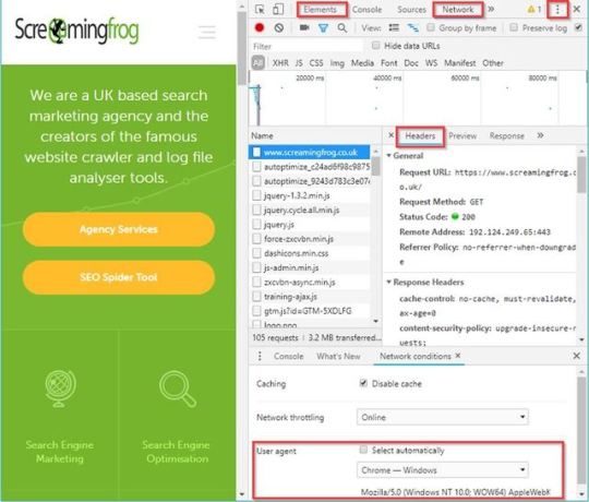
From crawl completion notifications to automated reporting: this post may not have Billy the Kid or Butch Cassidy, instead, here are a few of my most useful tools to combine with the SEO Spider, (just as exciting). We SEOs are extremely lucky—not just because we’re working in such an engaging and collaborative industry, but we have access to a plethora of online resources, conferences and SEO-based tools to lend a hand with almost any task you could think up. My favourite of which is, of course, the SEO Spider—after all, following Minesweeper Outlook, it’s likely the most used program on my work PC. However, a great programme can only be made even more useful when combined with a gang of other fantastic tools to enhance, compliment or adapt the already vast and growing feature set. While it isn’t quite the ragtag group from John Sturges’ 1960 cult classic, I’ve compiled the Magnificent Seven(ish) SEO tools I find useful to use in conjunction with the SEO Spider: Debugging in Chrome Developer Tools Chrome is the definitive king of browsers, and arguably one of the most installed programs on the planet. What’s more, it’s got a full suite of free developer tools built straight in—to load it up, just right-click on any page and hit inspect. Among many aspects, this is particularly handy to confirm or debunk what might be happening in your crawl versus what you see in a browser. For instance, while the Spider does check response headers during a crawl, maybe you just want to dig a bit deeper and view it as a whole? Well, just go to the Network tab, select a request and open the Headers sub-tab for all the juicy details: Perhaps you’ve loaded a crawl that’s only returning one or two results and you think JavaScript might be the issue? Well, just hit the three dots (highlighted above) in the top right corner, then click settings > debugger > disable JavaScript and refresh your page to see how it looks: Or maybe you just want to compare your nice browser-rendered HTML to that served back to the Spider? Just open the Spider and enable ‘JavaScript Rendering’ & ‘Store Rendered HTML’ in the configuration options (Configuration > Spider > Rendering/Advanced), then run your crawl. Once complete, you can view the rendered HTML in the bottom ‘View Source’ tab and compare with the rendered HTML in the ‘elements’ tab of Chrome. There are honestly far too many options in the Chrome developer toolset to list here, but it’s certainly worth getting your head around. Page Validation with a Right-Click Okay, I’m cheating a bit here as this isn’t one tool, rather a collection of several, but have you ever tried right-clicking a URL within the Spider? Well, if not, I’d recommend giving it a go—on top of some handy exports like the crawl path report and visualisations, there’s a ton of options to open that URL into several individual analysis & validation apps: Google Cache – See how Google is caching and storing your pages’ HTML. Wayback Machine – Compare URL changes over time. Other Domains on IP – See all domains registered to that IP Address. Open Robots.txt – Look at a site’s Robots. HTML Validation with W3C – Double-check all HTML is valid. PageSpeed Insights – Any areas to improve site speed? Structured Data Tester – Check all on-page structured data. Mobile-Friendly Tester – Are your pages mobile-friendly? Rich Results Tester – Is the page eligible for rich results? AMP Validator – Official AMP project validation test. User Data and Link Metrics via API Access We SEOs can’t get enough data, it’s genuinely all we crave – whether that’s from user testing, keyword tracking or session information, we want it all and we want it now! After all, creating the perfect website for bots is one thing, but ultimately the aim of almost every site is to get more users to view and convert on the domain, so we need to view it from as many angles as possible. Starting with users, there’s practically no better insight into user behaviour than the raw data provided by both Google Search Console (GSC) and Google Analytics (GA), both of which help us make informed, data-driven decisions and recommendations. What’s great about this is you can easily integrate any GA or GSC data straight into your crawl via the API Access menu so it’s front and centre when reviewing any changes to your pages. Just head on over to Configuration > API Access > [your service of choice], connect to your account, configure your settings and you’re good to go. Another crucial area in SERP rankings is the perceived authority of each page in the eyes of search engines – a major aspect of which, is (of course), links., links and more links. Any SEO will know you can’t spend more than 5 minutes at BrightonSEO before someone brings up the subject of links, it’s like the lifeblood of our industry. Whether their importance is dying out or not there’s no denying that they currently still hold much value within our perceptions of Google’s algorithm. Well, alongside the previous user data you can also use the API Access menu to connect with some of the biggest tools in the industry such as Moz, Ahrefs or Majestic, to analyse your backlink profile for every URL pulled in a crawl. For all the gory details on API Access check out the following page (scroll down for other connections): https://www.screamingfrog.co.uk/seo-spider/user-guide/configuration/ Understanding Bot Behaviour with the Log File Analyzer An often-overlooked exercise, nothing gives us quite the insight into how bots are interacting through a site than directly from the server logs. The trouble is, these files can be messy and hard to analyse on their own, which is where our very own Log File Analyzer (LFA) comes into play, (they didn’t force me to add this one in, promise!). I’ll leave @ScreamingFrog to go into all the gritty details on why this tool is so useful, but my personal favourite aspect is the ‘Import URL data’ tab on the far right. This little gem will effectively match any spreadsheet containing URL information with the bot data on those URLs. So, you can run a crawl in the Spider while connected to GA, GSC and a backlink app of your choice, pulling the respective data from each URL alongside the original crawl information. Then, export this into a spreadsheet before importing into the LFA to get a report combining metadata, session data, backlink data and bot data all in one comprehensive summary, aka the holy quadrilogy of technical SEO statistics. While the LFA is a paid tool, there’s a free version if you want to give it a go. Crawl Reporting in Google Data Studio One of my favourite reports from the Spider is the simple but useful ‘Crawl Overview’ export (Reports > Crawl Overview), and if you mix this with the scheduling feature, you’re able to create a simple crawl report every day, week, month or year. This allows you to monitor and for any drastic changes to the domain and alerting to anything which might be cause for concern between crawls. However, in its native form it’s not the easiest to compare between dates, which is where Google Sheets & Data Studio can come in to lend a hand. After a bit of setup, you can easily copy over the crawl overview into your master G-Sheet each time your scheduled crawl completes, then Data Studio will automatically update, letting you spend more time analysing changes and less time searching for them. This will require some fiddling to set up; however, at the end of this section I’ve included links to an example G-Sheet and Data Studio report that you’re welcome to copy. Essentially, you need a G-Sheet with date entries in one column and unique headings from the crawl overview report (or another) in the remaining columns: Once that’s sorted, take your crawl overview report and copy out all the data in the ‘Number of URI’ column (column B), being sure to copy from the ‘Total URI Encountered’ until the end of the column. Open your master G-Sheet and create a new date entry in column A (add this in a format of YYYYMMDD). Then in the adjacent cell, Right-click > ‘Paste special’ > ‘Paste transposed’ (Data Studio prefers this to long-form data): If done correctly with several entries of data, you should have something like this: Once the data is in a G-Sheet, uploading this to Data Studio is simple, just create a new report > add data source > connect to G-Sheets > [your master sheet] > [sheet page] and make sure all the heading entries are set as a metric (blue) while the date is set as a dimension (green), like this: You can then build out a report to display your crawl data in whatever format you like. This can include scorecards and tables for individual time periods, or trend graphs to compare crawl stats over the date range provided, (you’re very own Search Console Coverage report). Here’s an overview report I quickly put together as an example. You can obviously do something much more comprehensive than this should you wish, or perhaps take this concept and combine it with even more reports and exports from the Spider. If you’d like a copy of both my G-Sheet and Data Studio report, feel free to take them from here: Master Crawl Overview G-Sheet: https://docs.google.com/spreadsheets/d/1FnfN8VxlWrCYuo2gcSj0qJoOSbIfj7bT9ZJgr2pQcs4/edit?usp=sharing Crawl Overview Data Studio Report: https://datastudio.google.com/open/1Luv7dBnkqyRj11vLEb9lwI8LfAd0b9Bm Note: if you take a copy some of the dimension formats may change within DataStudio (breaking the graphs), so it’s worth checking the date dimension is still set to ‘Date (YYYMMDD)’ Building Functions & Strings with XPath Helper & Regex Search The Spider is capable of doing some very cool stuff with the extraction feature, a lot of which is listed in our guide to web scraping and extraction. The trouble with much of this is it will require you to build your own XPath or regex string to lift your intended information. While simply right-clicking > Copy XPath within the inspect window will usually do enough to scrape, by it’s not always going to cut it for some types of data. This is where two chrome extensions, XPath Helper & Regex- Search come in useful. Unfortunately, these won’t automatically build any strings or functions, but, if you combine them with a cheat sheet and some trial and error you can easily build one out in Chrome before copying into the Spider to bulk across all your pages. For example, say I wanted to get all the dates and author information of every article on our blog subfolder (https://www.screamingfrog.co.uk/blog/). If you simply right clicked on one of the highlighted elements in the inspect window and hit Copy > Copy XPath, you would be given something like: /html/body/div[4]/div/div[1]/div/div[1]/div/div[1]/p While this does the trick, it will only pull the single instance copied (‘16 January, 2019 by Ben Fuller’). Instead, we want all the dates and authors from the /blog subfolder. By looking at what elements the reference is sitting in we can slowly build out an XPath function directly in XPath Helper and see what it highlights in Chrome. For instance, we can see it sits in a class of ‘main-blog–posts_single-inner–text–inner clearfix’, so pop that as a function into XPath Helper: //div[@class="main-blog--posts_single-inner--text--inner clearfix"] XPath Helper will then highlight the matching results in Chrome: Close, but this is also pulling the post titles, so not quite what we’re after. It looks like the date and author names are sitting in a sub

tag so let’s add that into our function: (//div[@class="main-blog--posts_single-inner--text--inner clearfix"])/p Bingo! Stick that in the custom extraction feature of the Spider (Configuration > Custom > Extraction), upload your list of pages, and watch the results pour in! Regex Search works much in the same way: simply start writing your string, hit next and you can visually see what it’s matching as you’re going. Once you got it, whack it in the Spider, upload your URLs then sit back and relax. Notifications & Auto Mailing Exports with Zapier Zapier brings together all kinds of web apps, letting them communicate and work with one another when they might not otherwise be able to. It works by having an action in one app set as a trigger and another app set to perform an action as a result. To make things even better, it works natively with a ton of applications such as G-Suite, Dropbox, Slack, and Trello. Unfortunately, as the Spider is a desktop app, we can’t directly connect it with Zapier. However, with a bit of tinkering, we can still make use of its functionality to provide email notifications or auto mailing reports/exports to yourself and a list of predetermined contacts whenever a scheduled crawl completes. All you need is to have your machine or server set up with an auto cloud sync directory such as those on ‘Dropbox’, ‘OneDrive’ or ‘Google Backup & Sync’. Inside this directory, create a folder to save all your crawl exports & reports. In this instance, I’m using G-drive, but others should work just as well. You’ll need to set a scheduled crawl in the Spider (file > Schedule) to export any tabs, bulk exports or reports into a timestamped folder within this auto-synced directory: Log into or create an account for Zapier and make a new ‘zap’ to email yourself or a list of contacts whenever a new folder is generated within the synced directory you selected in the previous step. You’ll have to provide Zapier access to both your G-Drive & Gmail for this to work (do so at your own risk). My zap looks something like this: The above Zap will trigger when a new folder is added to /Scheduled Crawls/ in my G-Drive account. It will then send out an email from my Gmail to myself and any other contacts, notifying them and attaching a direct link to the newly added folder and Spider exports. I’d like to note here that if running a large crawl or directly saving the crawl file to G-drive, you’ll need enough storage to upload (so I’d stick to exports). You’ll also have to wait until the sync is completed from your desktop to the cloud before the zap will trigger, and it checks this action on a cycle of 15 minutes, so might not be instantaneous. Alternatively, do the same thing on IFTTT (If This Then That) but set it so a new G-drive file will ping your phone, turn your smart light a hue of lime green or just play this sound at full volume on your smart speaker. We really are living in the future now! Conclusion There you have it, the Magnificent Seven(ish) tools to try using with the SEO Spider, combined to form the deadliest gang in the west web. Hopefully, you find some of these useful, but I’d love to hear if you have any other suggestions to add to the list. The post SEO Spider Companion Tools, Aka ‘The Magnificent Seven’ appeared first on Screaming Frog.

#google-analytics-integration

0 notes

onlinemarketingcourses · 6 years ago

Text

Using Python to recover SEO site traffic (Part three) Search Engine Watch

When you incorporate machine learning techniques to speed up SEO recovery, the results can be amazing.

As mentioned before, you can find the code used in part one, two and three in this Google Colab notebook.

Let’s get started.

URL matching vs content matching

Fortunately, it is possible to group pages by their contents because most page templates have different content structures. They serve different user needs, so that needs to be the case.

How can we organize pages by their content? We can use DOM element selectors for this. We will specifically use XPaths.

A scientist’s bottom-up approach

One of the reasons I advocate practitioners learn programming is that you can start solving problems using your domain expertise and find shortcuts like the one I will share next.

Hamlet’s observation and a simpler solution

For most ecommerce sites, most page templates include images (and input elements), and those generally change in quantity and size.

Now let’s get to the fun part and get to code some machine learning code in Python!

Collecting training data

In our case, as discussed above, we’ll use our intuition that most product pages have one or more large images on the page, and most category type pages have many smaller images on the page.

What’s more, product pages typically have more form elements than category pages (for filling in quantity, color, and more).

Here we load the raw data already collected.

Feature engineering

Each row of the form_counts data frame above corresponds to a single URL and provides a count of both form elements, and input elements contained on that page.

Most site pages can have an arbitrary number of images. We are going to further process our dataset by bucketing images into 50 groups. This technique is called “binning”.

Here is what our processed data set looks like.

Adding ground truth labels

As we already have correct labels from our manual regex approach, we can use them to create the correct labels to feed the model.

Model training and grid search

Finally, the good stuff!

All the steps above, the data collection and preparation, are generally the hardest part to code. The machine learning code is generally quite simple.

Evaluating performance

In order to understand where the model performs best and worst, we will use another useful machine learning tool, the confusion matrix.

Here is the code to put together the confusion matrix:

Finally, here is the code to plot the model evaluation:

Resources to learn more

You might be thinking that this is a lot of work to just tell page groups, and you are right!

If you want to jump onto the machine learning bandwagon, here are some resources I recommend to learn more:

Got any tips or queries? Share it in the comments.

Hamlet Batista is the CEO and founder of RankSense, an agile SEO platform for online retailers and manufacturers. He can be found on Twitter .

Want to stay on top of the latest search trends?

Get top insights and news from our search experts.