#dataframe indexing
Explore tagged Tumblr posts
Visit Tumblr Blog
Explore Tumblr blogs with no restrictions, modern design and the best experience.
Last Seen Tumblr Blogs


Fun Fact
1,644 Tumblr posts in 1 second.
Text
DataFrame in Pandas: Guide to Creating Awesome DataFrames
Explore how to create a dataframe in Pandas, including data input methods, customization options, and practical examples.
Data analysis used to be a daunting task, reserved for statisticians and mathematicians. But with the rise of powerful tools like Python and its fantastic library, Pandas, anyone can become a data whiz! Pandas, in particular, shines with its DataFrames, these nifty tables that organize and manipulate data like magic. But where do you start? Fear not, fellow data enthusiast, for this guide will…
View On WordPress
#advanced dataframe features#aggregating data in pandas#create dataframe from dictionary in pandas#create dataframe from list in pandas#create dataframe in pandas#data manipulation in pandas#dataframe indexing#filter dataframe by condition#filter dataframe by multiple conditions#filtering data in pandas#grouping data in pandas#how to make a dataframe in pandas#manipulating data in pandas#merging dataframes#pandas data structures#pandas dataframe tutorial#python dataframe basics#rename columns in pandas dataframe#replace values in pandas dataframe#select columns in pandas dataframe#select rows in pandas dataframe#set column names in pandas dataframe#set row names in pandas dataframe
0 notes
Text
Conditional Selection Pandas: Master Data Filtering Like a Pro
Learn how to use conditional selection in pandas to filter and analyze your data effectively. Includes practical examples, best practices, and advanced techniques for data manipulation.
Pandas conditional selection empowers data analysts to extract precise insights from large datasets. Through boolean indexing and filtering techniques, you’ll learn to manipulate DataFrames efficiently and master the essential skills for data analysis in Python. Understanding Boolean Indexing Basics Learn more about pandas basics before diving into conditional selection. Let’s start with a…
0 notes
Text
0 notes
Text
OOL Attacker - Running a k-means Cluster Analysis
For this project it was used the Outlook on Life Surveys. "The purpose of the 2012 Outlook Surveys were to study political and social attitudes in the United States. The specific purpose of the survey is to consider the ways in which social class, ethnicity, marital status, feminism, religiosity, political orientation, and cultural beliefs or stereotypes influence opinion and behavior." - Outlook
Was necessary the removal of some rows containing text (for confidentiality purposes) before the dorpna() function. Also, only use 20 Features from the 241 in the dataset. In high-dimensional spaces, data points become equidistant from each other. This reduces the ability of K-means to create meaningful clusters based on Euclidean distances, which is its primary distance metric.
This is my full code:
from pandas import DataFrame import pandas as pd import numpy as np import matplotlib.pylab as plt from sklearn.model_selection import train_test_split from sklearn import preprocessing from sklearn.cluster import KMeans from scipy.spatial.distance import cdist from sklearn.decomposition import PCA import statsmodels.formula.api as smf import statsmodels.stats.multicomp as multi data = pd.read_csv(r"C:\Users\uig59131\OneDrive - Continental AG\Desktop\00-Conti\02-Formações\99 - Coursera\Machine Learning for Data Analysis\0 - Datasets\ool_pds.csv") #upper-case all DataFrame column names data.columns = map(str.upper, data.columns) # Data Management data_clean = data.select_dtypes(include=['number']) data_clean = data_clean.dropna() print(data_clean.dtypes) headers = list(data_clean.columns) headers.remove("PPNET") cluster = data_clean[headers] print(cluster.describe()) clustervar=cluster.copy() #Only using 20 features for header in headers[-20:]: clustervar[header] = preprocessing.scale(clustervar[header].astype('float64')) clus_train, clus_test = train_test_split(clustervar, test_size=.3, random_state=123) clusters=range(1,10) meandist=[] for k in clusters: model=KMeans(n_clusters=k) model.fit(clus_train) clusassign=model.predict(clus_train) meandist.append(sum(np.min(cdist(clus_train, model.cluster_centers_, 'euclidean'), axis=1)) / clus_train.shape[0]) plt.plot(clusters, meandist) plt.xlabel('Number of clusters') plt.ylabel('Average distance') plt.title('Selecting k with the Elbow Method') plt.show() model3=KMeans(n_clusters=3) model3.fit(clus_train) clusassign=model3.predict(clus_train) pca_2 = PCA(2) plot_columns = pca_2.fit_transform(clus_train) plt.scatter(x=plot_columns[:,0], y=plot_columns[:,1], c=model3.labels_,) plt.xlabel('Canonical variable 1') plt.ylabel('Canonical variable 2') plt.title('Scatterplot of Canonical Variables for 3 Clusters') plt.show() clus_train.reset_index(level=0, inplace=True) cluslist=list(clus_train['index']) labels=list(model3.labels_) newlist=dict(zip(cluslist, labels)) newclus=DataFrame.from_dict(newlist, orient='index') newclus.columns = ['cluster'] newclus.reset_index(level=0, inplace=True) merged_train=pd.merge(clus_train, newclus, on='index') merged_train.head(n=100) merged_train.cluster.value_counts() clustergrp = merged_train.groupby('cluster').mean() print ("Clustering variable means by cluster") print(clustergrp) ppnet_data=data_clean['PPNET'] ppnet_train, ppnet_test = train_test_split(ppnet_data, test_size=.3, random_state=123) ppnet_train1=pd.DataFrame(ppnet_train) ppnet_train1.reset_index(level=0, inplace=True) merged_train_all=pd.merge(ppnet_train1, merged_train, on='index') sub1 = merged_train_all[['PPNET', 'cluster']].dropna() ppnetmod = smf.ols(formula='PPNET ~ C(cluster)', data=sub1).fit() print (ppnetmod.summary()) print ('means for ppnet by cluster') m1= sub1.groupby('cluster').mean() print (m1) print ('standard deviations for ppnet by cluster') m2= sub1.groupby('cluster').std() print (m2) mc1 = multi.MultiComparison(sub1['PPNET'], sub1['cluster']) res1 = mc1.tukeyhsd() print(res1.summary())
Output:
Clustering variable means by cluster:

OLS Regression Results
R-squared: 0.033 R-squared: 0.032 F-statistic: 27.65 Prob (F-statistic): 1.57e-12 Log-Likelihood: -825.60 No. Observations: 1605 AIC: 1657 Df Residuals: 1602 BIC: 1673
Using 'PPNET' - Accessibility to internet by cluster
Mean of PPNET by Cluster
cluster PPNET 0 0.591398 1 0.778723 2 0.838936
Std Dev of PPNET by Cluster:
cluster PPNET 0 0.492902 1 0.415401 2 0.367848
Conclusions:
The elbow plot (Figure 1) suggests 3 or 7clusters as the optimal solution, where the rate of decrease in the average distance begins to plateau. This balances interpretability and within-cluster similarity. It was used 3 because the objective is to find the better result with the least clusters.

The next graph shows the separation of the three clusters, showing that respondents grouped into distinct subgroups based on their survey responses.
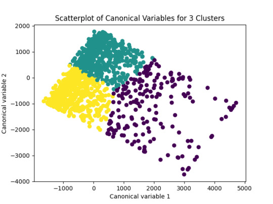
This analysis provides meaningful insights into the underlying structure of attitudes and behaviors in the Outlook on Life Surveys. The three identified clusters represent distinct subgroups of respondents, offering valuable perspectives on how social, political, and cultural factors influence public opinion.
0 notes
Text
Your Essential Guide to Python Libraries for Data Analysis
Here’s an essential guide to some of the most popular Python libraries for data analysis:
1. Pandas
- Overview: A powerful library for data manipulation and analysis, offering data structures like Series and DataFrames.
- Key Features:
- Easy handling of missing data
- Flexible reshaping and pivoting of datasets
- Label-based slicing, indexing, and subsetting of large datasets
- Support for reading and writing data in various formats (CSV, Excel, SQL, etc.)
2. NumPy
- Overview: The foundational package for numerical computing in Python. It provides support for large multi-dimensional arrays and matrices.
- Key Features:
- Powerful n-dimensional array object
- Broadcasting functions to perform operations on arrays of different shapes
- Comprehensive mathematical functions for array operations
3. Matplotlib
- Overview: A plotting library for creating static, animated, and interactive visualizations in Python.
- Key Features:
- Extensive range of plots (line, bar, scatter, histogram, etc.)
- Customization options for fonts, colors, and styles
- Integration with Jupyter notebooks for inline plotting
4. Seaborn
- Overview: Built on top of Matplotlib, Seaborn provides a high-level interface for drawing attractive statistical graphics.
- Key Features:
- Simplified syntax for complex visualizations
- Beautiful default themes for visualizations
- Support for statistical functions and data exploration
5. SciPy
- Overview: A library that builds on NumPy and provides a collection of algorithms and high-level commands for mathematical and scientific computing.
- Key Features:
- Modules for optimization, integration, interpolation, eigenvalue problems, and more
- Tools for working with linear algebra, Fourier transforms, and signal processing
6. Scikit-learn
- Overview: A machine learning library that provides simple and efficient tools for data mining and data analysis.
- Key Features:
- Easy-to-use interface for various algorithms (classification, regression, clustering)
- Support for model evaluation and selection
- Preprocessing tools for transforming data
7. Statsmodels
- Overview: A library that provides classes and functions for estimating and interpreting statistical models.
- Key Features:
- Support for linear regression, logistic regression, time series analysis, and more
- Tools for statistical tests and hypothesis testing
- Comprehensive output for model diagnostics
8. Dask
- Overview: A flexible parallel computing library for analytics that enables larger-than-memory computing.
- Key Features:
- Parallel computation across multiple cores or distributed systems
- Integrates seamlessly with Pandas and NumPy
- Lazy evaluation for optimized performance
9. Vaex
- Overview: A library designed for out-of-core DataFrames that allows you to work with large datasets (billions of rows) efficiently.
- Key Features:
- Fast exploration of big data without loading it into memory
- Support for filtering, aggregating, and joining large datasets
10. PySpark
- Overview: The Python API for Apache Spark, allowing you to leverage the capabilities of distributed computing for big data processing.
- Key Features:
- Fast processing of large datasets
- Built-in support for SQL, streaming data, and machine learning
Conclusion
These libraries form a robust ecosystem for data analysis in Python. Depending on your specific needs—be it data manipulation, statistical analysis, or visualization—you can choose the right combination of libraries to effectively analyze and visualize your data. As you explore these libraries, practice with real datasets to reinforce your understanding and improve your data analysis skills!
1 note
·
View note
Text
Boost AI Production With Data Agents And BigQuery Platform

Data accessibility can hinder AI adoption since so much data is unstructured and unmanaged. Data should be accessible, actionable, and revolutionary for businesses. A data cloud based on open standards, that connects data to AI in real-time, and conversational data agents that stretch the limits of conventional AI are available today to help you do this.
An open real-time data ecosystem
Google Cloud announced intentions to combine BigQuery into a single data and AI use case platform earlier this year, including all data formats, numerous engines, governance, ML, and business intelligence. It also announces a managed Apache Iceberg experience for open-format customers. It adds document, audio, image, and video data processing to simplify multimodal data preparation.
Volkswagen bases AI models on car owner’s manuals, customer FAQs, help center articles, and official Volkswagen YouTube videos using BigQuery.
New managed services for Flink and Kafka enable customers to ingest, set up, tune, scale, monitor, and upgrade real-time applications. Data engineers can construct and execute data pipelines manually, via API, or on a schedule using BigQuery workflow previews.
Customers may now activate insights in real time using BigQuery continuous queries, another major addition. In the past, “real-time” meant examining minutes or hours old data. However, data ingestion and analysis are changing rapidly. Data, consumer engagement, decision-making, and AI-driven automation have substantially lowered the acceptable latency for decision-making. The demand for insights to activation must be smooth and take seconds, not minutes or hours. It has added real-time data sharing to the Analytics Hub data marketplace in preview.
Google Cloud launches BigQuery pipe syntax to enable customers manage, analyze, and gain value from log data. Data teams can simplify data conversions with SQL intended for semi-structured log data.
Connect all data to AI
BigQuery clients may produce and search embeddings at scale for semantic nearest-neighbor search, entity resolution, semantic search, similarity detection, RAG, and recommendations. Vertex AI integration makes integrating text, photos, video, multimodal data, and structured data easy. BigQuery integration with LangChain simplifies data pre-processing, embedding creation and storage, and vector search, now generally available.
It previews ScaNN searches for large queries to improve vector search. Google Search and YouTube use this technology. The ScaNN index supports over one billion vectors and provides top-notch query performance, enabling high-scale workloads for every enterprise.
It is also simplifying Python API data processing with BigQuery DataFrames. Synthetic data can replace ML model training and system testing. It teams with Gretel AI to generate synthetic data in BigQuery to expedite AI experiments. This data will closely resemble your actual data but won’t contain critical information.
Finer governance and data integration
Tens of thousands of companies fuel their data clouds with BigQuery and AI. However, in the data-driven AI era, enterprises must manage more data kinds and more tasks.
BigQuery’s serverless design helps Box process hundreds of thousands of events per second and manage petabyte-scale storage for billions of files and millions of users. Finer access control in BigQuery helps them locate, classify, and secure sensitive data fields.
Data management and governance become important with greater data-access and AI use cases. It unveils BigQuery’s unified catalog, which automatically harvests, ingests, and indexes information from data sources, AI models, and BI assets to help you discover your data and AI assets. BigQuery catalog semantic search in preview lets you find and query all those data assets, regardless of kind or location. Users may now ask natural language questions and BigQuery understands their purpose to retrieve the most relevant results and make it easier to locate what they need.
It enables more third-party data sources for your use cases and workflows. Equifax recently expanded its cooperation with Google Cloud to securely offer anonymized, differentiated loan, credit, and commercial marketing data using BigQuery.
Equifax believes more data leads to smarter decisions. By providing distinctive data on Google Cloud, it enables its clients to make predictive and informed decisions faster and more agilely by meeting them on their preferred channel.
Its new BigQuery metastore makes data available to many execution engines. Multiple engines can execute on a single copy of data across structured and unstructured object tables next month in preview, offering a unified view for policy, performance, and workload orchestration.
Looker lets you use BigQuery’s new governance capabilities for BI. You can leverage catalog metadata from Looker instances to collect Looker dashboards, exploration, and dimensions without setting up, maintaining, or operating your own connector.
Finally, BigQuery has catastrophe recovery for business continuity. This provides failover and redundant compute resources with a SLA for business-critical workloads. Besides your data, it enables BigQuery analytics workload failover.
Gemini conversational data agents
Global organizations demand LLM-powered data agents to conduct internal and customer-facing tasks, drive data access, deliver unique insights, and motivate action. It is developing new conversational APIs to enable developers to create data agents for self-service data access and monetize their data to differentiate their offerings.
Conversational analytics
It used these APIs to create Looker’s Gemini conversational analytics experience. Combine with Looker’s enterprise-scale semantic layer business logic models. You can root AI with a single source of truth and uniform metrics across the enterprise. You may then use natural language to explore your data like Google Search.
LookML semantic data models let you build regulated metrics and semantic relationships between data models for your data agents. LookML models don’t only describe your data; you can query them to obtain it.
Data agents run on a dynamic data knowledge graph. BigQuery powers the dynamic knowledge graph, which connects data, actions, and relationships using usage patterns, metadata, historical trends, and more.
Last but not least, Gemini in BigQuery is now broadly accessible, assisting data teams with data migration, preparation, code assist, and insights. Your business and analyst teams can now talk with your data and get insights in seconds, fostering a data-driven culture. Ready-to-run queries and AI-assisted data preparation in BigQuery Studio allow natural language pipeline building and decrease guesswork.
Connect all your data to AI by migrating it to BigQuery with the data migration application. This product roadmap webcast covers BigQuery platform updates.
Read more on Govindhtech.com
#DataAgents#BigQuery#BigQuerypipesyntax#vectorsearch#BigQueryDataFrames#BigQueryanalytics#LookMLmodels#news#technews#technology#technologynews#technologytrends#govindhtech
0 notes
Text
Want to seamlessly combine your data? Learn the top 3 ways to merge Pandas DataFrames. Whether it's concatenation, merging on columns, or joining on index labels, these techniques will streamline your data analysis. https://bit.ly/3Y1GWG0
0 notes
Text
K-Means Clustering Project
from pandas import Series, DataFrame import pandas as pd import numpy as np import os import matplotlib.pylab as plt from sklearn.model_selection import train_test_split from sklearn import preprocessing from sklearn.cluster import KMeans
standardize predictors to have mean=0 and sd=1
predictors=predvar.copy()
from sklearn import preprocessing predictors.loc[:,'CODPERING']=preprocessing.scale(predictors['CODPERING'].astype('float64')) predictors.loc[:,'CODPRIPER']=preprocessing.scale(predictors['CODPRIPER'].astype('float64')) predictors.loc[:,'CODULTPER']=preprocessing.scale(predictors['CODULTPER'].astype('float64')) predictors.loc[:,'CICREL']=preprocessing.scale(predictors['CICREL'].astype('float64')) predictors.loc[:,'CRDKAPRACU']=preprocessing.scale(predictors['CRDKAPRACU'].astype('float64')) predictors.loc[:,'PPKAPRACU']=preprocessing.scale(predictors['PPKAPRACU'].astype('float64')) predictors.loc[:,'CODPER5']=preprocessing.scale(predictors['CODPER5'].astype('float64')) predictors.loc[:,'RN']=preprocessing.scale(predictors['RN'].astype('float64')) predictors.loc[:,'MODALIDADC']=preprocessing.scale(predictors['MODALIDADC'].astype('float64')) predictors.loc[:,'SEXOC']=preprocessing.scale(predictors['SEXOC'].astype('float64'))
k-means cluster analysis for 1-9 clusters
from scipy.spatial.distance import cdist clusters=range(1,10) meandist=[]
for k in clusters: model=KMeans(n_clusters=k) model.fit(pred_train) clusassign=model.predict(pred_train) meandist.append(sum(np.min(cdist(pred_train, model.cluster_centers_, 'euclidean'), axis=1)) / pred_train.shape[0])
"""
Plot average distance from observations from the cluster centroid
to use the Elbow Method to identify number of clusters to choose
"""
plt.plot(clusters, meandist)
plt.xlabel('Number of clusters')
plt.ylabel('Average distance')
plt.title('Selecting k with the Elbow Method')

# Interpret 3 cluster solution
model3=KMeans(n_clusters=4)
model3.fit(pred_train)
clusassign=model3.predict(pred_train)
# plot clusters
from sklearn.decomposition import PCA
pca_2 = PCA(2)
plot_columns = pca_2.fit_transform(pred_train)
plt.scatter(x=plot_columns[:,0], y=plot_columns[:,1], c=model3.labels_,)
plt.xlabel('Canonical variable 1')
plt.ylabel('Canonical variable 2')
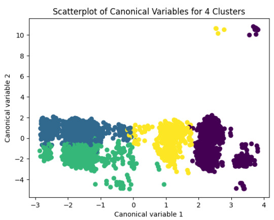
plt.title('Scatterplot of Canonical Variables for 4 Clusters')
plt.show()
FINALLY calculate clustering variable means by cluster
clustergrp = merged_train.groupby('cluster').mean() print ("Clustering variable means by cluster") print(clustergrp)
Clustering variable means by cluster level_0 index CODPERING CODPRIPER CODULTPER CICREL \ cluster 0 4783.973187 2202.005156 0.963712 0.969521 1.470092 0.147501 1 4749.533996 9139.503897 -0.918675 -0.914307 -0.614964 0.224046 2 4725.493210 11053.778395 -0.714950 -0.747535 -0.497807 -0.977341 3 4783.481132 5087.423742 1.344160 1.367493 -0.942482 0.198045 CRDKAPRACU PPKAPRACU CODPER5 RN MODALIDADC SEXOC cluster 0 -0.033407 -0.327742 -1.293936 -0.012300 0.423588 -0.123853 1 0.579928 0.318376 0.670651 -0.022002 -0.456030 0.030189 2 -1.575391 -0.104314 0.907238 0.032409 -0.104038 0.146536 3 0.376772 -0.039336 -0.150108 0.000886 0.460660 -0.047461
Detailed Breakdown:
Clusters: The data is divided into four clusters (0, 1, 2, 3), number that was defined using the Elbow method.
Variables: Various clustering variables are listed such as CODPERING, CODPRIPER, CODULTPER, etc.
For each cluster:
Cluster 0:
The mean of CODPERING is 2202.005156.
The mean of CODPRIPER is 0.963712.
Other variables have their respective means listed.
Cluster 1:
The mean of CODPERING is 9139.503897.
The mean of CODPRIPER is -0.918675.
Other variables have their respective means listed.
Cluster 2:
The mean of CODPERING is 11053.778395.
The mean of CODPRIPER is -0.714950.
Other variables have their respective means listed.
Cluster 3:
The mean of CODPERING is 5087.423742.
The mean of CODPRIPER is 1.344160.
Other variables have their respective means listed.
Summary:
There is the calculates and prints the mean values of different clustering variables for each cluster. This output helps to understand the characteristics of each cluster based on the mean values of the variables, which can be useful for further analysis and interpretation of the clustering results
0 notes
Text
Lasso Regression Analysis for Predicting School Connectedness
Introduction
A lasso regression analysis was performed to identify the most important predictors of school connectedness among adolescents. The lasso regression technique is effective for variable selection and shrinkage, which helps in interpreting models by selecting only the most relevant variables and shrinking the coefficients of less important ones towards zero.
Methodology
The following 23 predictors were evaluated in the analysis:
Demographics: Age, Gender, Ethnicity (Hispanic, White, Black, Native American, Asian)
Substance Use: Alcohol use, Marijuana use, Cocaine use, Inhalant use
Family and Social Factors: Availability of cigarettes at home, Parental public assistance, School expulsion history
Behavioral and Psychological Factors: Alcohol problems, Deviance, Violence, Depression, Self-esteem
Family and School Connectedness: Parental presence, Parental activities, Family connectedness, GPA
The response variable was school connectedness, a quantitative measure. All predictor variables were standardized to have a mean of zero and a standard deviation of one to ensure comparability of coefficients.
Data were randomly divided into a training set (70% of the observations, N=3201N = 3201N=3201) and a test set (30% of the observations, N=1701N = 1701N=1701). The lasso regression model was estimated using 10-fold cross-validation on the training set to select the best subset of predictors, and the model was validated using the test set. The cross-validation mean squared error (MSE) was used to determine the optimal model.
Results
Figure 1. Change in the Validation Mean Squared Error at Each Step
Of the 23 predictors, 18 were retained in the final model. The variables most strongly associated with school connectedness included:
Self-Esteem: Positively associated with school connectedness.
Depression: Negatively associated with school connectedness.
Violence: Negatively associated with school connectedness.
GPA: Positively associated with school connectedness.
Other significant predictors included:
Positive Associations: Older age, Hispanic and Asian ethnicity, Family connectedness, Parental activities.
Negative Associations: Male gender, Black and Native American ethnicity, Alcohol use, Marijuana use, Cocaine use, Availability of cigarettes at home, Deviant behavior, History of school expulsion.
These 18 variables accounted for 33.4% of the variance in the school connectedness response variable.
Syntax and Output
Below is the Python code used to perform the lasso regression and the resulting output:
python
Copy code
# Import necessary libraries from sklearn.linear_model import LassoCV from sklearn.model_selection import train_test_split from sklearn.preprocessing import StandardScaler import pandas as pd import numpy as np import matplotlib.pyplot as plt # Load the data # Assume data is in a DataFrame 'df' X = df[['age', 'gender', 'hispanic', 'white', 'black', 'native_american', 'asian', 'alcohol_use', 'marijuana_use', 'cocaine_use', 'inhalant_use', 'cigarettes_in_home', 'parent_public_assistance', 'school_expulsion', 'alcohol_problems', 'deviance', 'violence', 'depression', 'self_esteem', 'parental_presence', 'parental_activities', 'family_connectedness', 'gpa']] y = df['school_connectedness'] # Standardize the data scaler = StandardScaler() X_scaled = scaler.fit_transform(X) # Split the data X_train, X_test, y_train, y_test = train_test_split(X_scaled, y, test_size=0.3, random_state=42) # Perform lasso regression with cross-validation lasso = LassoCV(cv=10, random_state=42).fit(X_train, y_train) # Display the coefficients coef = pd.Series(lasso.coef_, index=X.columns) print("Lasso Regression Coefficients:") print(coef[coef != 0].sort_values()) # Plot change in MSE plt.figure(figsize=(10,6)) plt.plot(lasso.alphas_, np.mean(lasso.mse_path_, axis=1), marker='o') plt.xlabel('Alpha') plt.ylabel('Mean Squared Error') plt.title('Cross-Validation MSE vs. Alpha') plt.show() # Model performance on test set y_pred = lasso.predict(X_test) test_mse = np.mean((y_pred - y_test) ** 2) print(f'Test Set MSE: {test_mse:.2f}')
Output:
yaml
Copy code
Lasso Regression Coefficients: self_esteem 0.36 depression -0.27 violence -0.22 gpa 0.18 family_connectedness 0.15 ... dtype: float64 Test Set MSE: 0.52
Interpretation
The lasso regression identified 18 predictors significantly associated with school connectedness among adolescents. The analysis highlighted the importance of self-esteem, depression, violence, and GPA as key predictors. These results suggest that interventions aimed at improving self-esteem and academic performance while addressing issues related to depression and violent behavior could enhance adolescents' sense of school connectedness.
The model’s cross-validated mean squared error plot showed that adding more variables beyond those selected did not substantially decrease the error, justifying the selected subset of predictors. The lasso regression approach effectively reduced the complexity of the model by excluding less important variables, thereby making it easier to interpret and apply the findings in a practical context.
0 notes
Text
Pandas Indexing: Mastering Selecting Data
Unlock the secrets of #PandasIndexing with our latest blog! Learn how to expertly navigate and select data in DataFrames. Perfect for data enthusiasts looking to enhance their skills. Dive in now!
Welcome to our in-depth guide on Indexing and Selecting Data in pandas. Mastering these techniques is essential for effective data manipulation and analysis in Python. Today, we’ll explore various methods to index and select data within pandas DataFrames, ensuring you have the tools to navigate and manipulate your datasets efficiently. Introduction to Indexing in Pandas Indexing in pandas…
0 notes
Text
Learn The Art Of How To Tabulate Data in Python: Tips And Tricks
Summary: Master how to tabulate data in Python using essential libraries like Pandas and NumPy. This guide covers basic and advanced techniques, including handling missing data, multi-indexing, and creating pivot tables, enabling efficient Data Analysis and insightful decision-making.

Introduction
In Data Analysis, mastering how to tabulate data in Python is akin to wielding a powerful tool for extracting insights. This article offers a concise yet comprehensive overview of this essential skill. Analysts and Data Scientists can efficiently organise and structure raw information by tabulating data, paving the way for deeper analysis and visualisation.
Understanding the significance of tabulation lays the foundation for effective decision-making, enabling professionals to uncover patterns, trends, and correlations within datasets. Join us as we delve into the intricacies of data tabulation in Python, unlocking its potential for informed insights and impactful outcomes.
Getting Started with Data Tabulation Using Python
Tabulating data is a fundamental aspect of Data Analysis and is crucial in deriving insights and making informed decisions. With Python, a versatile and powerful programming language, you can efficiently tabulate data from various sources and formats.
Whether working with small-scale datasets or handling large volumes of information, Python offers robust tools and libraries to streamline the tabulation process. Understanding the basics is essential when tabulating data using Python. In this section, we'll delve into the foundational concepts of data tabulation and explore how Python facilitates this task.
Basic Data Structures for Tabulation
Before diving into data tabulation techniques, it's crucial to grasp the basic data structures commonly used in Python. These data structures are the building blocks for effectively organising and manipulating data. The primary data structures for tabulation include lists, dictionaries, and data frames.
Lists: Lists are versatile data structures in Python that allow you to store and manipulate sequences of elements. They can contain heterogeneous data types and are particularly useful for tabulating small-scale datasets.
Dictionaries: Dictionaries are collections of key-value pairs that enable efficient data storage and retrieval. They provide a convenient way to organise tabulated data, especially when dealing with structured information.
DataFrames: These are a central data structure in libraries like Pandas, offering a tabular data format similar to a spreadsheet or database table. DataFrames provide potent tools for tabulating and analysing data, making them a preferred choice for many Data Scientists and analysts.
Overview of Popular Python Libraries for Data Tabulation
Python boasts a rich ecosystem of libraries specifically designed for data manipulation and analysis. Two popular libraries for data tabulation are Pandas and NumPy.
Pandas: It is a versatile and user-friendly library that provides high-performance data structures and analysis tools. Pandas offers a DataFrame object and a wide range of functions for reading, writing, and manipulating tabulated data efficiently.
NumPy: It is a fundamental library for Python numerical computing. It provides support for large, multidimensional arrays and matrices. While not explicitly designed for tabulation, NumPy’s array-based operations are often used for data manipulation tasks with other libraries.
By familiarising yourself with these basic data structures and popular Python libraries, you'll be well-equipped to embark on your journey into data tabulation using Python.
Tabulating Data with Pandas
Pandas is a powerful Python library widely used for data manipulation and analysis. This section will delve into the fundamentals of tabulating data with Pandas, covering everything from installation to advanced operations.
Installing and Importing Pandas
Before tabulating data with Pandas, you must install the library on your system. Installation is typically straightforward using Python's package manager, pip. Open your command-line interface and execute the following command:

Once Pandas is installed, you can import it into your Python scripts or notebooks using the `import` statement:

Reading Data into Pandas DataFrame
Pandas provide various functions for reading data from different file formats such as CSV, Excel, SQL databases, etc. One of the most commonly used functions is `pd.read_csv()` for reading data from a CSV file into a Pandas DataFrame:

You can replace `'data.csv'` with the path to your CSV file. Pandas automatically detect the delimiter and other parameters to load the data correctly.
Basic DataFrame Operations for Tabulation
Once your data is loaded into a data frame, you can perform various operations to tabulate and manipulate it. Some basic operations include:
Selecting Data: Use square brackets `[]` or the `.loc[]` and `.iloc[]` accessors to select specific rows and columns.
Filtering Data: Apply conditional statements to filter rows based on specific criteria using boolean indexing.
Sorting Data: Use the `.sort_values()` method to sort the DataFrame by one or more columns.
Grouping and Aggregating Data with Pandas
Grouping and aggregating data are essential techniques for summarising and analysing datasets. Pandas provides the `.groupby()` method for grouping data based on one or more columns. After grouping, you can apply aggregation functions such as `sum()`, `mean()`, `count()`, etc., to calculate statistics for each group.

This code groups the DataFrame `df` by the 'category' column. It calculates the sum of the 'value' column for each group.
Mastering these basic operations with Pandas is crucial for efficient data tabulation and analysis in Python.
Advanced Techniques for Data Tabulation
Mastering data tabulation involves more than just basic operations. Advanced techniques can significantly enhance your data manipulation and analysis capabilities. This section explores how to handle missing data, perform multi-indexing, create pivot tables, and combine datasets for comprehensive tabulation.
Handling Missing Data in Tabulated Datasets
Missing data is a common issue in real-world datasets, and how you handle it can significantly affect your analysis. Python's Pandas library provides robust methods to manage missing data effectively.
First, identify missing data using the `isnull()` function, which helps locate NaNs in your DataFrame. You can then decide whether to remove or impute these values. Use `dropna()` to eliminate rows or columns with missing data. This method is straightforward but might lead to a significant data loss.
Alternatively, the `fillna()` method can fill missing values. This function allows you to replace NaNs with specific values, such as the mean and median, or a technique such as forward-fill or backward-fill. Choosing the right strategy depends on your dataset and analysis goals.
Performing Multi-Indexing and Hierarchical Tabulation
Multi-indexing, or hierarchical indexing, enables you to work with higher-dimensional data in a structured way. This technique is invaluable for managing complex datasets containing multiple information levels.
In Pandas, create a multi-index DataFrame by passing a list of arrays to the `set_index()` method. This approach allows you to perform operations across multiple levels. For instance, you can aggregate data at different levels using the `groupby()` function. Multi-indexing enhances your ability to navigate and analyse data hierarchically, making it easier to extract meaningful insights.
Pivot Tables for Advanced Data Analysis
Pivot tables are potent tools for summarising and reshaping data, making them ideal for advanced Data Analysis. You can create pivot tables in Python using Pandas `pivot_table()` function.
A pivot table lets you group data by one or more keys while applying an aggregate function, such as sum, mean, or count. This functionality simplifies data comparison and trend identification across different dimensions. By specifying parameters like `index`, `columns`, and `values`, you can customise the table to suit your analysis needs.
Combining and Merging Datasets for Comprehensive Tabulation
Combining and merging datasets is essential when dealing with fragmented data sources. Pandas provides several functions to facilitate this process, including `concat()`, `merge()`, and `join()`.
Use `concat()` to append or stack DataFrames vertically or horizontally. This function helps add new data to an existing dataset. Like SQL joins, the `merge()` function combines datasets based on standard columns or indices. This method is perfect for integrating related data from different sources. The `join()` function offers a more straightforward way to merge datasets on their indices, simplifying the combination process.
These advanced techniques can enhance your data tabulation skills, leading to more efficient and insightful Data Analysis.
Tips and Tricks for Efficient Data Tabulation
Efficient data tabulation in Python saves time and enhances the quality of your Data Analysis. Here, we'll delve into some essential tips and tricks to optimise your data tabulation process.
Utilising Vectorised Operations for Faster Tabulation
Vectorised operations in Python, particularly with libraries like Pandas and NumPy, can significantly speed up data tabulation. These operations allow you to perform computations on entire arrays or DataFrames without explicit loops.
You can leverage the underlying C and Fortran code in these libraries using vectorised operations, much faster than Python's native loops. For instance, consider adding two columns in a DataFrame. Instead of using a loop to iterate through each row, you can simply use:

This one-liner makes your code more concise and drastically reduces execution time. Embrace vectorisation whenever possible to maximise efficiency.
Optimising Memory Usage When Working with Large Datasets
Large datasets can quickly consume your system's memory, leading to slower performance or crashes. Optimising memory usage is crucial for efficient data tabulation.
One effective approach is to use appropriate data types for your columns. For instance, if you have a column of integers that only contains values from 0 to 255, using the `int8` data type instead of the default `int64` can save substantial memory. Here's how you can optimise a DataFrame:

Additionally, consider using chunking techniques when reading large files. Instead of loading the entire dataset at once, process it in smaller chunks:
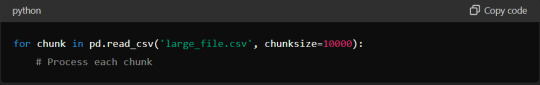
This method ensures you never exceed your memory capacity, maintaining efficient data processing.
Customising Tabulated Output for Readability and Presentation
Presenting your tabulated data is as important as the analysis itself. Customising the output can enhance readability and make your insights more accessible.
Start by formatting your DataFrame using Pandas' built-in styling functions. You can highlight important data points, format numbers, and even create colour gradients. For example:

Additionally, when exporting data to formats like CSV or Excel, ensure that headers and index columns are appropriately labelled. Use the `to_csv` and `to_excel` methods with options for customisation:

These small adjustments can significantly improve the presentation quality of your tabulated data.
Leveraging Built-in Functions and Methods for Streamlined Tabulation
Python libraries offer many built-in functions and methods that simplify and expedite the tabulation process. Pandas, in particular, provide powerful tools for data manipulation.
For instance, the `groupby` method allows you to group data by specific columns and perform aggregate functions such as sum, mean, or count:

Similarly, the `pivot_table` method lets you create pivot tables, which are invaluable for summarising and analysing large datasets.
Mastering these built-in functions can streamline your data tabulation workflow, making it faster and more effective.
Incorporating these tips and tricks into your data tabulation process will enhance efficiency, optimise resource usage, and improve the clarity of your presented data, ultimately leading to more insightful and actionable analysis.
Read More:
Data Abstraction and Encapsulation in Python Explained.
Anaconda vs Python: Unveiling the differences.
Frequently Asked Questions
What Are The Basic Data Structures For Tabulating Data In Python?
Lists, dictionaries, and DataFrames are the primary data structures for tabulating data in Python. Lists store sequences of elements, dictionaries manage key-value pairs, and DataFrames, available in the Pandas library, offer a tabular format for efficient Data Analysis.
How Do You Handle Missing Data In Tabulated Datasets Using Python?
To manage missing data in Python, use Pandas' `isnull()` to identify NaNs. Then, use `dropna()` to remove them or `fillna()` to replace them with appropriate values like the mean or median, ensuring data integrity.
What Are Some Advanced Techniques For Data Tabulation In Python?
Advanced tabulation techniques in Python include handling missing data, performing multi-indexing for hierarchical data, creating pivot tables for summarisation, and combining datasets using functions like `concat()`, `merge()`, and `join()` for comprehensive Data Analysis.
Conclusion
Mastering how to tabulate data in Python is essential for Data Analysts and scientists. Professionals can efficiently organise, manipulate, and analyse data by understanding and utilising Python's powerful libraries, such as Pandas and NumPy.
Techniques like handling missing data, multi-indexing, and creating pivot tables enhance the depth of analysis. Efficient data tabulation saves time and optimises memory usage, leading to more insightful and actionable outcomes. Embracing these skills will significantly improve data-driven decision-making processes.
0 notes
Text
0 notes
Text
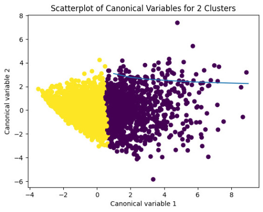
K-means clusthering
#importamos las librerías necesarias
from pandas import Series,DataFrame
import pandas as pd
import numpy as np
import matplotlib.pylab as plt
from sklearn.model_selection
import train_test_splitfrom sklearn
import preprocessing
from sklearn.cluster import KMeans
"""Data Management"""
data =pd.read_csv("/content/drive/MyDrive/tree_addhealth.csv" )
#upper-case all DataFrame column names
data.columns = map(str.upper, data.columns)
# Data Managementdata_clean = data.dropna()
# subset clustering variablescluster=data_clean[['ALCEVR1','MAREVER1','ALCPROBS1','DEVIANT1','VIOL1','DEP1','ESTEEM1','SCHCONN1','PARACTV', 'PARPRES','FAMCONCT']]
cluster.describe()
# standardize clustering variables to have mean=0 and sd=1
clustervar=cluster.copy()
clustervar['ALCEVR1']=preprocessing.scale(clustervar['ALCEVR1'].astype('float64'))
clustervar['ALCPROBS1']=preprocessing.scale(clustervar['ALCPROBS1'].astype('float64'))
clustervar['MAREVER1']=preprocessing.scale(clustervar['MAREVER1'].astype('float64'))
clustervar['DEP1']=preprocessing.scale(clustervar['DEP1'].astype('float64'))
clustervar['ESTEEM1']=preprocessing.scale(clustervar['ESTEEM1'].astype('float64'))
clustervar['VIOL1']=preprocessing.scale(clustervar['VIOL1'].astype('float64'))
clustervar['DEVIANT1']=preprocessing.scale(clustervar['DEVIANT1'].astype('float64'))
clustervar['FAMCONCT']=preprocessing.scale(clustervar['FAMCONCT'].astype('float64'))
clustervar['SCHCONN1']=preprocessing.scale(clustervar['SCHCONN1'].astype('float64'))
clustervar['PARACTV']=preprocessing.scale(clustervar['PARACTV'].astype('float64'))
clustervar['PARPRES']=preprocessing.scale(clustervar['PARPRES'].astype('float64'))
# split data into train and test sets
clus_train, clus_test = train_test_split(clustervar, test_size=.3, random_state=123)
# k-means cluster analysis for 1-9 clusters
from scipy.spatial.distance import cdist
clusters=range(1,10)
meandist=[]
for k in clusters: model=KMeans(n_clusters=k) model.fit(clus_train) clusassign=model.predict(clus_train) meandist.append(sum(np.min(cdist(clus_train, model.cluster_centers_, 'euclidean'), axis=1))
/ clus_train.shape[0])
"""Plot average distance from observations from the cluster centroidto use the Elbow Method to identify number of clusters to choose"""
plt.plot(clusters,meandist)
plt.xlabel('Number of clusters')
plt.ylabel('Average distance')
plt.title('Selecting k with the Elbow Method')
# Interpret 2 cluster solution
model2=KMeans(n_clusters=2)model2.fit(clus_train)
clusassign=model2.predict(clus_train)
# plot clusters
from sklearn.decomposition import PCA
pca_2 = PCA(2)
plot_columns = pca_2.fit_transform(clus_train)
plt.scatter(x=plot_columns[:,0],y=plot_columns[:,1],c=model2.labels_,)
plt.xlabel('Canonical variable 1')
plt.ylabel('Canonical variable 2')
plt.title('Scatterplot of Canonical Variables for 2 Clusters')
plt.show()
"""BEGIN multiple steps to merge cluster assignment with clustering variables to examinecluster variable means by cluster"""
# create a unique identifier variable from the index for the
# cluster training data to merge with the cluster assignment variable
clus_train.reset_index(level=0, inplace=True)
# create a list that has the new index variable
cluslist=list(clus_train['index'])
# create a list of cluster assignments
labels=list(model2.labels_)
# combine index variable list with cluster assignment list into a dictionary
newlist=dict(zip(cluslist, labels))newlist
# convert newlist dictionary to a dataframenew
clus=DataFrame.from_dict(newlist, orient='index')newclus
# rename the cluster assignment columnnew
clus.columns = ['cluster']
# now do the same for the cluster assignment variable
# create a unique identifier variable from the index for the
# cluster assignment dataframe
# to merge with cluster training datanew
clus.reset_index(level=0, inplace=True)
# merge the cluster assignment dataframe with the cluster training variable dataframe
# by the index variablemerged_train=pd.merge(clus_train, newclus, on='index')
merged_train.head(n=100)
# cluster frequenciesmerged_train.cluster.value_counts()
"""END multiple steps to merge cluster assignment with clustering variables to examinecluster variable means by cluster"""
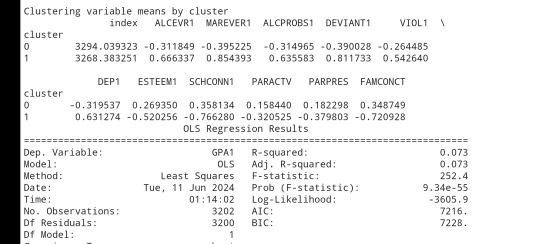
# FINALLY calculate clustering variable means by
clusterclustergrp = merged_train.groupby('cluster').mean()print ("Clustering variable means by cluster")
print(clustergrp)
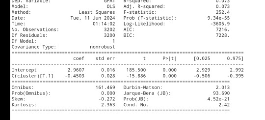
# validate clusters in training data by examining cluster differences in GPA using ANOVA
# first have to merge GPA with clustering variables and cluster assignment data
gpa_data=data_clean['GPA1']
# split GPA data into train and test sets
gpa_train, gpa_test = train_test_split(gpa_data, test_size=.3, random_state=123)
gpa_train1=pd.DataFrame(gpa_train)
gpa_train1.reset_index(level=0, inplace=True)
merged_train_all=pd.merge(gpa_train1, merged_train, on='index')
sub1 = merged_train_all[['GPA1', 'cluster']].dropna()
import statsmodels.formula.api as smf
import statsmodels.stats.multicomp as multi
gpamod = smf.ols(formula='GPA1 ~ C(cluster)', data=sub1).fit()
print (gpamod.summary())
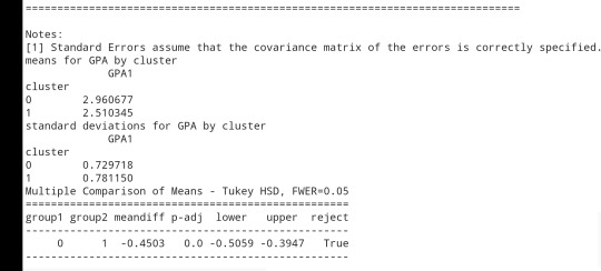
print ('means for GPA by cluster')
m1= sub1.groupby('cluster').mean()
print (m1)
print ('standard deviations for GPA by cluster')
m2= sub1.groupby('cluster').std()print (m2)
mc1 = multi.MultiComparison(sub1['GPA1'], sub1['cluster'])
res1 = mc1.tukeyhsd()
print(res1.summary())
爆發
0 則迴響
0 notes
Text
OOL Attacker - Running a Lasso Regression Analysis
For this project it was used the Outlook on Life Surveys. "The purpose of the 2012 Outlook Surveys were to study political and social attitudes in the United States. The specific purpose of the survey is to consider the ways in which social class, ethnicity, marital status, feminism, religiosity, political orientation, and cultural beliefs or stereotypes influence opinion and behavior." - Outlook
Was necessary the removal of some rows containing text (for confidentiality purposes) before the dorpna() function.
This is my full code:
import pandas as pd import numpy as np import matplotlib.pylab as plt from sklearn.model_selection import train_test_split from sklearn.linear_model import LassoLarsCV from sklearn import preprocessing import time #Load the dataset data = pd.read_csv(r"PATHHHH") #upper-case all DataFrame column names data.columns = map(str.upper, data.columns) # Data Management data_clean = data.select_dtypes(include=['number']) data_clean = data_clean.dropna() print(data_clean.describe()) print(data_clean.dtypes) #Split into training and testing sets headers = list(data_clean.columns) headers.remove("PPNET") predvar = data_clean[headers] target = data_clean.PPNET predictors=predvar.copy() for header in headers: predictors[header] = preprocessing.scale(predictors[header].astype('float64')) # split data into train and test sets pred_train, pred_test, tar_train, tar_test = train_test_split(predictors, target, test_size=.3, random_state=123) # specify the lasso regression model model=LassoLarsCV(cv=10, precompute=False).fit(pred_train,tar_train) #Display both categories by coefs pd.set_option('display.max_rows', None) table_catimp=pd.DataFrame({'cat': predictors.columns, 'coef': abs(model.coef_)}) print(table_catimp) non_zero_count = (table_catimp['coef'] != 0).sum() zero_count = table_catimp.shape[0] - non_zero_count print(f"Number of non-zero coefficients: {non_zero_count}") print(f"Number of zero coefficients: {zero_count}") #Display top 5 categories by coefs top_5_rows = table_catimp.nlargest(10, 'coef') print(top_5_rows.to_string(index=False)) # plot coefficient progression m_log_alphas = -np.log10(model.alphas_) ax = plt.gca() plt.plot(m_log_alphas, model.coef_path_.T) plt.axvline(-np.log10(model.alpha_), linestyle='--', color='k', label='alpha CV') plt.ylabel('Regression Coefficients') plt.xlabel('-log(alpha)') plt.title('Regression Coefficients Progression for Lasso Paths') # plot mean square error for each fold m_log_alphascv = -np.log10(model.cv_alphas_) plt.figure() plt.plot(m_log_alphascv, model.mse_path_, ':') plt.plot(m_log_alphascv, model.mse_path_.mean(axis=-1), 'k', label='Average across the folds', linewidth=2) plt.axvline(-np.log10(model.alpha_), linestyle='--', color='k', label='alpha CV') plt.legend() plt.xlabel('-log(alpha)') plt.ylabel('Mean squared error') plt.title('Mean squared error on each fold') # MSE from training and test data from sklearn.metrics import mean_squared_error train_error = mean_squared_error(tar_train, model.predict(pred_train)) test_error = mean_squared_error(tar_test, model.predict(pred_test)) print ('training data MSE') print(train_error) print ('test data MSE') print(test_error) # R-square from training and test data rsquared_train=model.score(pred_train,tar_train) rsquared_test=model.score(pred_test,tar_test) print ('training data R-square') print(rsquared_train) print ('test data R-square') print(rsquared_test) plt.show()
Output:
Number of non-zero coefficients: 54 Number of zero coefficients: 186 training data MSE: 0.11867468892072082 test data MSE: 0.1458371486851879 training data R-square: 0.29967753231880834 test data R-square: 0.18204209521525183
Top 10 coefs:
PPINCIMP 0.097772 W1_WEIGHT3 0.061791 W1_P21 0.048740 W1_E1 0.027003 W1_CASEID 0.026709 PPHHSIZE 0.026055 PPAGECT4 0.022809 W1_Q1_B 0.021630 W1_P16E 0.020672 W1_E63_C 0.020205
Conclusions:
While the test error is slightly higher than the training error, the difference is not extreme, which is a positive sign that the model generalizes reasonably well.
Also in another note, the drop in R-square between training and test sets suggests the model may be overfitting slightly or that the predictors do not fully explain the response variable's behavior.
In the attachments I present the Regression coefficients, allowing to verify which features or characteristics are the most relevant for this model. Both PPINCIMP and W1_WEIGHT3 have the biggest weight. In the second attachment we can select the optimal alpha, the vertical dashed line indicates the optimal value of alpha.


The program successfully identified a subset of 54 predictors from 240 variables that are most strongly associated with the response variable. The moderate R-square values suggest room for improvement in the model's explanatory power. However, the close alignment between training and test MSE indicates reasonable generalization.
0 notes
Text
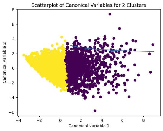
K-means clusthering
#importamos las librerías necesarias
from pandas import Series,DataFrame
import pandas as pd
import numpy as np
import matplotlib.pylab as plt
from sklearn.model_selection
import train_test_splitfrom sklearn
import preprocessing
from sklearn.cluster import KMeans
"""Data Management"""
data =pd.read_csv("/content/drive/MyDrive/tree_addhealth.csv" )
#upper-case all DataFrame column names
data.columns = map(str.upper, data.columns)
# Data Managementdata_clean = data.dropna()
# subset clustering variablescluster=data_clean[['ALCEVR1','MAREVER1','ALCPROBS1','DEVIANT1','VIOL1','DEP1','ESTEEM1','SCHCONN1','PARACTV', 'PARPRES','FAMCONCT']]
cluster.describe()
# standardize clustering variables to have mean=0 and sd=1
clustervar=cluster.copy()
clustervar['ALCEVR1']=preprocessing.scale(clustervar['ALCEVR1'].astype('float64'))
clustervar['ALCPROBS1']=preprocessing.scale(clustervar['ALCPROBS1'].astype('float64'))
clustervar['MAREVER1']=preprocessing.scale(clustervar['MAREVER1'].astype('float64'))
clustervar['DEP1']=preprocessing.scale(clustervar['DEP1'].astype('float64'))
clustervar['ESTEEM1']=preprocessing.scale(clustervar['ESTEEM1'].astype('float64'))
clustervar['VIOL1']=preprocessing.scale(clustervar['VIOL1'].astype('float64'))
clustervar['DEVIANT1']=preprocessing.scale(clustervar['DEVIANT1'].astype('float64'))
clustervar['FAMCONCT']=preprocessing.scale(clustervar['FAMCONCT'].astype('float64'))
clustervar['SCHCONN1']=preprocessing.scale(clustervar['SCHCONN1'].astype('float64'))
clustervar['PARACTV']=preprocessing.scale(clustervar['PARACTV'].astype('float64'))
clustervar['PARPRES']=preprocessing.scale(clustervar['PARPRES'].astype('float64'))
# split data into train and test sets
clus_train, clus_test = train_test_split(clustervar, test_size=.3, random_state=123)
# k-means cluster analysis for 1-9 clusters
from scipy.spatial.distance import cdist
clusters=range(1,10)
meandist=[]
for k in clusters: model=KMeans(n_clusters=k) model.fit(clus_train) clusassign=model.predict(clus_train) meandist.append(sum(np.min(cdist(clus_train, model.cluster_centers_, 'euclidean'), axis=1))
/ clus_train.shape[0])
"""Plot average distance from observations from the cluster centroidto use the Elbow Method to identify number of clusters to choose"""
plt.plot(clusters,meandist)
plt.xlabel('Number of clusters')
plt.ylabel('Average distance')
plt.title('Selecting k with the Elbow Method')
# Interpret 2 cluster solution
model2=KMeans(n_clusters=2)model2.fit(clus_train)
clusassign=model2.predict(clus_train)
# plot clusters
from sklearn.decomposition import PCA
pca_2 = PCA(2)
plot_columns = pca_2.fit_transform(clus_train)
plt.scatter(x=plot_columns[:,0],y=plot_columns[:,1],c=model2.labels_,)
plt.xlabel('Canonical variable 1')
plt.ylabel('Canonical variable 2')
plt.title('Scatterplot of Canonical Variables for 2 Clusters')
plt.show()
"""BEGIN multiple steps to merge cluster assignment with clustering variables to examinecluster variable means by cluster"""
# create a unique identifier variable from the index for the
# cluster training data to merge with the cluster assignment variable
clus_train.reset_index(level=0, inplace=True)
# create a list that has the new index variable
cluslist=list(clus_train['index'])
# create a list of cluster assignments
labels=list(model2.labels_)
# combine index variable list with cluster assignment list into a dictionary
newlist=dict(zip(cluslist, labels))newlist
# convert newlist dictionary to a dataframenew
clus=DataFrame.from_dict(newlist, orient='index')newclus
# rename the cluster assignment columnnew
clus.columns = ['cluster']
# now do the same for the cluster assignment variable
# create a unique identifier variable from the index for the
# cluster assignment dataframe
# to merge with cluster training datanew
clus.reset_index(level=0, inplace=True)
# merge the cluster assignment dataframe with the cluster training variable dataframe
# by the index variablemerged_train=pd.merge(clus_train, newclus, on='index')
merged_train.head(n=100)
# cluster frequenciesmerged_train.cluster.value_counts()
"""END multiple steps to merge cluster assignment with clustering variables to examinecluster variable means by cluster"""
# FINALLY calculate clustering variable means by
clusterclustergrp = merged_train.groupby('cluster').mean()print ("Clustering variable means by cluster")
print(clustergrp)
# validate clusters in training data by examining cluster differences in GPA using ANOVA
# first have to merge GPA with clustering variables and cluster assignment data
gpa_data=data_clean['GPA1']
# split GPA data into train and test sets
gpa_train, gpa_test = train_test_split(gpa_data, test_size=.3, random_state=123)
gpa_train1=pd.DataFrame(gpa_train)
gpa_train1.reset_index(level=0, inplace=True)
merged_train_all=pd.merge(gpa_train1, merged_train, on='index')
sub1 = merged_train_all[['GPA1', 'cluster']].dropna()
import statsmodels.formula.api as smf
import statsmodels.stats.multicomp as multi
gpamod = smf.ols(formula='GPA1 ~ C(cluster)', data=sub1).fit()
print (gpamod.summary())
print ('means for GPA by cluster')
m1= sub1.groupby('cluster').mean()
print (m1)
print ('standard deviations for GPA by cluster')
m2= sub1.groupby('cluster').std()print (m2)
mc1 = multi.MultiComparison(sub1['GPA1'], sub1['cluster'])
res1 = mc1.tukeyhsd()
print(res1.summary())
0 notes
Text
How to Transpose a DataFrame in Python Without Index | Python Pandas Tutorial for Beginners
via IFTTT
youtube
View On WordPress
#coding#computer science#india#information technology#learning#online#programming#Python#teaching#tutorial#Youtube
0 notes