#and it's a covariance function..
Explore tagged Tumblr posts
Text
i still don't really get what a kernel is and at this point i'm afraid to ask
#basically i should know more math.#they've come up in quantum (aka the propagator) and stats and while i tried to understand i have not succeeded#you can expand a kernel into its basis functions.. or go from the basis functions to a kernel..#and it's a covariance function..#or a green's function which is kinda the same/similar?#i just. dont really know where it came from. it was presented to us very much like we should already know what it is
66 notes
·
View notes
Text
A Short Intro to Category Theory
A common theme in mathematics is to study certain objects and the maps between that preserve the specific structure of said objects. For example, linear algebra is the study of vector spaces and linear maps. Often we have that the identity maps are structure preserving and the composition of maps is also structure preserving. In the case of vector spaces, the identity map is a linear map and the composition of linear maps is again a linear map. Category theory generalises and axiomatises this common way of studying mathematical objects.
I'll introduce the notion of a category as well as the notion of a functor, which is another very important and ubiquitous notion in category theory. And I will finish with a very powerful result involving functors and isomorphisms!
Definition 1:
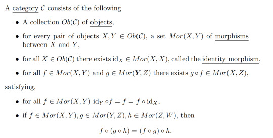
We call the last property the associative property.
Here are some examples:
Examples 2:

Note that whilst all of these examples are built from sets and set functions, we can have other kinds of objects and morphisms. However the most common categories are those built from Set.
Functors:
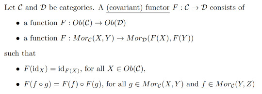
In the spirit of category theory being the study of objects and their morphisms, we want to define some kind of map between categories. It turns out that these are very powerful and show up everywhere in pure maths. Naturally, we want a functor to map objects to objects and morphisms to morphisms in a way that respects identity morphisms and our associative property.
Definition 3:
Example 4:
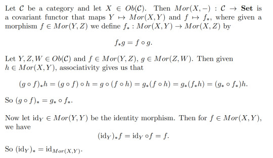
For those familiar with a some topology, the fundamental group is another exmaple of a covariant functor from the category of based spaces and based maps to Grp.
We also have another kind of functor:
Defintion 5:
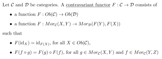
It may seem a bit odd to introduce at first since all we've done is swap the directions of the morphisms, but it turns out that contravariant functors show up a lot!
This example requires a little bit of knowledge of linear algebra.
Example 6:
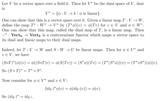
In fact, this is somewhat related to example 5! We can produce a contravariant functor Mor(-,X) is a similar way. For V and W vector spaces over k, we have that Mor(V,W) is a vector space over k. In particular, V*=Mor(V,k). So really this -* functor is just Mor(-,k)!
Isomorphisms
Here we generalise the familiar notion of isomorphisms of any algebraic structure!
Definition 7:
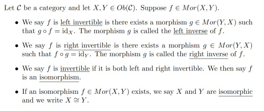
For a category of algebraic objects like Vectₖ, isomorphism are exactly the same as isomorphisms defined the typical way. In Top the isomorphisms are homeomorphisms. In Set the isomorphisms are bijective maps.
Remark:

So if f is invertible, we call it's right (or left) inverse, g, the inverse of f.
Isomorphisms give us a way to say when two objects of a category are "the same". More formally, being isomorphic defines an equivalence relation.
Lemma 8:
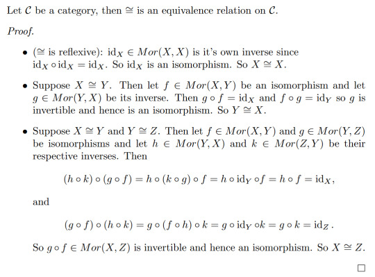
A natural question one might as is how do functors interact with isomorphisms? The answer is the very important result I hinted at in the intro!
Theorem 9:
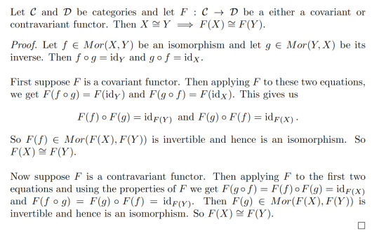
Remark: In general, the converse is not true. That is F(X) isomorphic to F(Y) does not imply X is isomorphic to Y. An example of this is the fundamental groups of both S² and ℝ² are isomorphic to the trivial group but these spaces are not homeomorphic.
Taking the negation of Theorem 9 gives us a very powerful result:
Corollary 10:

This means that if we can find a functor such that F(X) and F(Y) aren't isomorphic, we know that X and Y are not isomorphic. This is of particular importance in algebraic topology where we construct functors from Top or hTop to a category of a given algebraic structure. This gives us some very powerful topological invariants for telling when two spaces aren't homeomorphic or homotopy equivalent. (In fact, this is where category theory originated from!)
78 notes
·
View notes
Text
Reference archived on our website
Highlights • Long-COVID is heterogeneous in its symptoms, severity, and illness duration. • There was no association between long-COVID and cognitive performance. • Cognitive symptoms may represent functional cognitive disorders. • Long-COVID had lower mean diffusivity on diffusion imaging than normal recovery. • Diffusion imaging differences may suggest gliosis as a mechanism of long-COVID.
To be clear: There was no cognitive difference between people post infection. I can see some people misunderstanding what this says. It says there is some form of brain damage from covid across the board, even if you don't have long covid symptoms or diagnosis.
Abstract
Background
The pathophysiology of protracted symptoms after COVID-19 is unclear. This study aimed to determine if long-COVID is associated with differences in baseline characteristics, markers of white matter diffusivity in the brain, and lower scores on objective cognitive testing.
Methods
Individuals who experienced COVID-19 symptoms for more than 60 days post-infection (long-COVID) (n = 56) were compared to individuals who recovered from COVID-19 within 60 days of infection (normal recovery) (n = 35). Information regarding physical and mental health, and COVID-19 illness was collected. The National Institute of Health Toolbox Cognition Battery was administered. Participants underwent magnetic resonance imaging (MRI) with diffusion tensor imaging (DTI). Tract-based spatial statistics were used to perform a whole-brain voxel-wise analysis on standard DTI metrics (fractional anisotropy, axial diffusivity, mean diffusivity, radial diffusivity), controlling for age and sex. NIH Toolbox Age-Adjusted Fluid Cognition Scores were used to compare long-COVID and normal recovery groups, covarying for Age-Adjusted Crystallized Cognition Scores and years of education. False discovery rate correction was applied for multiple comparisons.
Results
There were no significant differences in age, sex, or history of neurovascular risk factors between the groups. The long-COVID group had significantly (p < 0.05) lower mean diffusivity than the normal recovery group across multiple white matter regions, including the internal capsule, anterior and superior corona radiata, corpus callosum, superior fronto-occiptal fasciculus, and posterior thalamic radiation. However, the effect sizes of these differences were small (all <|0.3|) and no significant differences were found for the other DTI metrics. Fluid cognition composite scores did not differ significantly between the long-COVID and normal recovery groups (p > 0.05).
Conclusions
Differences in diffusivity between long-COVID and normal recovery groups were found on only one DTI metric. This could represent subtle areas of pathology such as gliosis or edema, but the small effect sizes and non-specific nature of the diffusion indices make pathological inference difficult. Although long-COVID patients reported many neuropsychiatric symptoms, significant differences in objective cognitive performance were not found.
#long covid#covid 19#covid#mask up#pandemic#wear a mask#public health#coronavirus#sars cov 2#still coviding#wear a respirator#covid conscious#covid is not over
44 notes
·
View notes
Text
Hydrogen bomb vs. coughing baby: graphs and the Yoneda embedding
So we all love applying heavy duty theorems to prove easy results, right? One that caught my attention recently is a cute abstract way of defining graphs (specifically, directed multigraphs a.k.a. quivers). A graph G consists of the following data: a set G(V) of vertices, a set G(A) of arrows, and two functions G(s),G(t): G(A) -> G(V) which pick out the source and target vertex of an arrow. The notation I've used here is purposefully suggestive: the data of a graph is exactly the same as the data of a functor to the category of sets (call it Set) from the category that has two objects, and two parallel morphisms from one object to the other. We can represent this category diagrammatically as ∗⇉∗, but I am just going to call it Q.
The first object of Q we will call V, and the other we will call A. There will be two non-identity morphisms in Q, which we call s,t: V -> A. Note that s and t go from V to A, whereas G(s) and G(t) go from G(A) to G(V). We will define a graph to be a contravariant functor from Q to Set. We can encode this as a standard, covariant functor of type Q^op -> Set, where Q^op is the opposite category of Q. The reason to do this is that a graph is now exactly a presheaf on Q. Note that Q is isomorphic to its opposite category, so this change of perspective leaves the idea of a graph the same.
On a given small category C, the collection of all presheaves (which is in fact a proper class) has a natural structure as a category; the morphisms between two presheaves are the natural transformations between them. We call this category C^hat. In the case of C = Q, we can write down the data of such a natural transformations pretty easily. For two graphs G₁, G₂ in Q^hat, a morphism φ between them consists of a function φ_V: G₁(V) -> G₂(V) and a function φ_A: G₁(A) -> G₂(A). These transformations need to be natural, so because Q has two non-identity morphisms we require that two specific naturality squares commute. This gives us the equations G₂(s) ∘ φ_A = φ_V ∘ G₁(s) and G₂(t) ∘ φ_A = φ_V ∘ G₁(t). In other words, if you have an arrow in G₁ and φ_A maps it onto an arrow in G₂ and then you take the source/target of that arrow, it's the same as first taking the source/target in G₁ and then having φ_V map that onto a vertex of G₂. More explicitly, if v and v' are vertices in G₁(V) and a is an arrow from v to v', then φ_A(a) is an arrow from φ_V(v) to φ_V(v'). This is exactly what we want a graph homomorphism to be.
So Q^hat is the category of graphs and graph homomorphisms. This is where the Yoneda lemma enters the stage. If C is any (locally small) category, then an object C of C defines a presheaf on C in the following way. This functor (call it h_C for now) maps an object X of C onto the set of morphisms Hom(X,C) and a morphism f: X -> Y onto the function Hom(Y,C) -> Hom(X,C) given by precomposition with f. That is, for g ∈ Hom(Y,C) we have that the function h_C(f) maps g onto g ∘ f. This is indeed a contravariant functor from C to Set. Any presheaf that's naturally isomorphic to such a presheaf is called representable, and C is one of its representing objects.
So, if C is small, we have a function that maps objects of C onto objects of C^hat. Can we turn this into a functor C -> C^hat? This is pretty easy actually. For a given morphism f: C -> C' we need to find a natural transformation h_C -> h_C'. I.e., for every object X we need a set function ψ_X: Hom(X,C) -> Hom(X,C') (this is the X-component of the natural transformation) such that, again, various naturality squares commute. I won't beat around the bush too much and just say that this map is given by postcomposition with f. You can do the rest of the verification yourself.
For any small category C we have constructed a (covariant) functor C -> C^hat. A consequence of the Yoneda lemma is that this functor is full and faithful (so we can interpret C as a full subcategory of C^hat). Call it the Yoneda embedding, and denote it よ (the hiragana for 'yo'). Another fact, which Wikipedia calls the density theorem, is that any presheaf on C is, in a canonical way, a colimit (which you can think of as an abstract version of 'quotient of a disjoint union') of representable presheaves. Now we have enough theory to have it tell us something about graphs that we already knew.
Our small category Q has two objects: V and A. They give us two presheaves on Q, a.k.a. graphs, namely よ(V) and よ(A). What are these graphs? Let's calculate. The functor よ(V) maps the object V onto the one point set Hom(V,V) (which contains only id_V) and it maps A onto the empty set Hom(A,V). This already tells us (without calculating the action of よ(V) on s and t) that the graph よ(V) is the graph that consists of a single vertex and no arrows. The functor よ(A) maps V onto the two point set Hom(V,A) and A onto the one point set Hom(A,A). Two vertices (s and t), one arrow (id_A). What does よ(A) do with the Q-morphisms s and t? It should map them onto the functions Hom(A,A) -> Hom(V,A) that map a morphism f onto f ∘ s and f ∘ t, respectively. Because Hom(A,A) contains only id_A, these are the functions that map it onto s and t in Hom(V,A), respectively. So the one arrow in よ(A)(A) has s in よ(A)(V) as its source and t as its target. We conclude that よ(A) is the graph with two vertices and one arrow from one to the other.
We have found the representable presheaves on Q. By the density theorem, any graph is a colimit of よ(V) and よ(A) in a canonical way. Put another way: any graph consists of vertices and arrows between them. I'm sure you'll agree that this was worth the effort.
#math#adventures in cat theory#oh btw bc よ is full and faithful there are exactly two graph homomorphisms よ(V) -> よ(A)#namely よ(s) and よ(t)#which pick out exactly the source and target vertex in よ(A)
97 notes
·
View notes
Text
Viyaasan Mahalingasivam, from the London School of Hygiene and Tropical Medicine, and colleagues examined whether kidney function decline accelerated after COVID-19 versus other respiratory infections in a cohort study using linked data from the Stockholm Creatinine Measurements Project between Feb. 1, 2018, and Jan. 1, 2022. Data were included for all hospitalized and nonhospitalized adults in the database with at least one estimated glomerular filtration rate (eGFR) measurement in the two years prior to a COVID-19 positive test result (134,565 individuals) or pneumonia diagnosis (35,987 individuals).
The median baseline eGFR was 94 and 79 mL/min/1.73 m2 for the COVID-19 and pneumonia cohorts, respectively. The researchers found that both infections demonstrated accelerated annual eGFR decline after adjustment for covariates, with a greater magnitude of decline seen after COVID-19 than pneumonia (3.4 and 2.3 percent, respectively). Among individuals hospitalized for COVID-19, the decline was more severe (5.4 percent) but was similar among those hospitalized for pneumonia.
"We therefore propose that people who were hospitalized for COVID-19 receive closer monitoring of kidney function to ensure prompt diagnosis and optimized management of chronic kidney disease to effectively prevent complications and further decline," the authors write.
11 notes
·
View notes
Text
Interesting Papers for Week 32, 2024
In and Out of Criticality? State-Dependent Scaling in the Rat Visual Cortex. Castro, D. M., Feliciano, T., de Vasconcelos, N. A. P., Soares-Cunha, C., Coimbra, B., Rodrigues, A. J., … Copelli, M. (2024). PRX Life, 2(2), 023008.
An event-termination cue causes perceived time to dilate. Choe, S., & Kwon, O.-S. (2024). Psychonomic Bulletin & Review, 31(2), 659–669.
Stimulus-dependent differences in cortical versus subcortical contributions to visual detection in mice. Cone, J. J., Mitchell, A. O., Parker, R. K., & Maunsell, J. H. R. (2024). Current Biology, 34(9), 1940-1952.e5.
Sexually dimorphic control of affective state processing and empathic behaviors. Fang, S., Luo, Z., Wei, Z., Qin, Y., Zheng, J., Zhang, H., … Li, B. (2024). Neuron, 112(9), 1498-1517.e8.
Post-retrieval stress impairs subsequent memory depending on hippocampal memory trace reinstatement during reactivation. Heinbockel, H., Wagner, A. D., & Schwabe, L. (2024). Science Advances, 10(18).
An effect that counts: Temporally contiguous action effect enhances motor performance. Karsh, N., Ahmad, Z., Erez, F., & Hadad, B.-S. (2024). Psychonomic Bulletin & Review, 31(2), 897–905.
Learning enhances representations of taste-guided decisions in the mouse gustatory insular cortex. Kogan, J. F., & Fontanini, A. (2024). Current Biology, 34(9), 1880-1892.e5.
Babbling opens the sensory phase for imitative vocal learning. Leitão, A., & Gahr, M. (2024). Proceedings of the National Academy of Sciences, 121(18), e2312323121.
Information flow between motor cortex and striatum reverses during skill learning. Lemke, S. M., Celotto, M., Maffulli, R., Ganguly, K., & Panzeri, S. (2024). Current Biology, 34(9), 1831-1843.e7.
Statistically inferred neuronal connections in subsampled neural networks strongly correlate with spike train covariances. Liang, T., & Brinkman, B. A. W. (2024). Physical Review E, 109(4), 044404.
Pre-acquired Functional Connectivity Predicts Choice Inconsistency. Madar, A., Kurtz-David, V., Hakim, A., Levy, D. J., & Tavor, I. (2024). Journal of Neuroscience, 44(18), e0453232024.
Alpha-band sensory entrainment improves audiovisual temporal acuity. Marsicano, G., Bertini, C., & Ronconi, L. (2024). Psychonomic Bulletin & Review, 31(2), 874–885.
Excitability mediates allocation of pre-configured ensembles to a hippocampal engram supporting contextual conditioned threat in mice. Mocle, A. J., Ramsaran, A. I., Jacob, A. D., Rashid, A. J., Luchetti, A., Tran, L. M., … Josselyn, S. A. (2024). Neuron, 112(9), 1487-1497.e6.
Incidentally encoded temporal associations produce priming in implicit memory. Mundorf, A. M. D., Uitvlugt, M. G., & Healey, M. K. (2024). Psychonomic Bulletin & Review, 31(2), 761–771.
Intrinsic and Synaptic Contributions to Repetitive Spiking in Dentate Granule Cells. Shu, W.-C., & Jackson, M. B. (2024). Journal of Neuroscience, 44(18), e0716232024.
Dynamic prediction of goal location by coordinated representation of prefrontal-hippocampal theta sequences. Wang, Y., Wang, X., Wang, L., Zheng, L., Meng, S., Zhu, N., … Ming, D. (2024). Current Biology, 34(9), 1866-1879.e6.
Calibrating Bayesian Decoders of Neural Spiking Activity. Wei 魏赣超, G., Tajik Mansouri زینب تاجیک منصوری, Z., Wang 王晓婧, X., & Stevenson, I. H. (2024). Journal of Neuroscience, 44(18), e2158232024.
Attribute amnesia as a product of experience-dependent encoding. Yan, N., & Anderson, B. A. (2024). Psychonomic Bulletin & Review, 31(2), 772–780.
A common format for representing spatial location in visual and motor working memory. Yousif, S. R., Forrence, A. D., & McDougle, S. D. (2024). Psychonomic Bulletin & Review, 31(2), 697–707.
Unified control of temporal and spatial scales of sensorimotor behavior through neuromodulation of short-term synaptic plasticity. Zhou, S., & Buonomano, D. V. (2024). Science Advances, 10(18).
#neuroscience#science#research#brain science#scientific publications#cognitive science#neurobiology#cognition#psychophysics#neurons#neural computation#neural networks#computational neuroscience
9 notes
·
View notes
Text
a Basic Linear Regression Model
What is linear regression?
Linear regression analysis is used to predict the value of a variable based on the value of another variable. The variable you want to predict is called the dependent variable. The variable you are using to predict the other variable's value is called the independent variable.
This form of analysis estimates the coefficients of the linear equation, involving one or more independent variables that best predict the value of the dependent variable. Linear regression fits a straight line or surface that minimizes the discrepancies between predicted and actual output values. There are simple linear regression calculators that use a “least squares” method to discover the best-fit line for a set of paired data. You then estimate the value of X (dependent variable)
n statistics, simple linear regression (SLR) is a linear regression model with a single explanatory variable.[1][2][3][4][5] That is, it concerns two-dimensional sample points with one independent variable and one dependent variable (conventionally, the x and y coordinates in a Cartesian coordinate system) and finds a linear function (a non-vertical straight line) that, as accurately as possible, predicts the dependent variable values as a function of the independent variable. The adjective simple refers to the fact that the outcome variable is related to a single predictor.
It is common to make the additional stipulation that the ordinary least squares (OLS) method should be used: the accuracy of each predicted value is measured by its squared residual (vertical distance between the point of the data set and the fitted line), and the goal is to make the sum of these squared deviations as small as possible. In this case, the slope of the fitted line is equal to the correlation between y and x corrected by the ratio of standard deviations of these variables. The intercept of the fitted line is such that the line passes through the center of mass (x, y) of the data points.
Formulation and computation
[edit]
This relationship between the true (but unobserved) underlying parameters α and β and the data points is called a linear regression model.
Here we have introduced
x¯ and y¯ as the average of the xi and yi, respectively
Δxi and Δyi as the deviations in xi and yi with respect to their respective means.
Expanded formulas
[edit]
Interpretation
[edit]
Relationship with the sample covariance matrix
[edit]
where
rxy is the sample correlation coefficient between x and y
sx and sy are the uncorrected sample standard deviations of x and y
sx2 and sx,y are the sample variance and sample covariance, respectively
Interpretation about the slope
[edit]
Interpretation about the intercept
Interpretation about the correlation
[edit]
Numerical properties
[edit]
The regression line goes through the center of mass point, (x¯,y¯), if the model includes an intercept term (i.e., not forced through the origin).
The sum of the residuals is zero if the model includes an intercept term:∑i=1nε^i=0.
The residuals and x values are uncorrelated (whether or not there is an intercept term in the model), meaning:∑i=1nxiε^i=0
The relationship between ρxy (the correlation coefficient for the population) and the population variances of y (σy2) and the error term of ϵ (σϵ2) is:[10]: 401 σϵ2=(1−ρxy2)σy2For extreme values of ρxy this is self evident. Since when ρxy=0 then σϵ2=σy2. And when ρxy=1 then σϵ2=0.
Statistical properties
[edit]
Description of the statistical properties of estimators from the simple linear regression estimates requires the use of a statistical model. The following is based on assuming the validity of a model under which the estimates are optimal. It is also possible to evaluate the properties under other assumptions, such as inhomogeneity, but this is discussed elsewhere.[clarification needed]
Unbiasedness
[edit]
Variance of the mean response
[edit]
where m is the number of data points.
Variance of the predicted response
[edit]
Further information: Prediction interval
Confidence intervals
[edit]
The standard method of constructing confidence intervals for linear regression coefficients relies on the normality assumption, which is justified if either:
the errors in the regression are normally distributed (the so-called classic regression assumption), or
the number of observations n is sufficiently large, in which case the estimator is approximately normally distributed.
The latter case is justified by the central limit theorem.
Normality assumption
[edit]


Asymptotic assumption
[edit]
The alternative second assumption states that when the number of points in the dataset is "large enough", the law of large numbers and the central limit theorem become applicable, and then the distribution of the estimators is approximately normal. Under this assumption all formulas derived in the previous section remain valid, with the only exception that the quantile t*n−2 of Student's t distribution is replaced with the quantile q* of the standard normal distribution. Occasionally the fraction 1/n−2 is replaced with 1/n. When n is large such a change does not alter the results appreciably.
Numerical example
[edit]
See also: Ordinary least squares § Example, and Linear least squares § Example
Alternatives
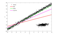
[edit]Calculating the parameters of a linear model by minimizing the squared error.
In SLR, there is an underlying assumption that only the dependent variable contains measurement error; if the explanatory variable is also measured with error, then simple regression is not appropriate for estimating the underlying relationship because it will be biased due to regression dilution.
Other estimation methods that can be used in place of ordinary least squares include least absolute deviations (minimizing the sum of absolute values of residuals) and the Theil–Sen estimator (which chooses a line whose slope is the median of the slopes determined by pairs of sample points).
Deming regression (total least squares) also finds a line that fits a set of two-dimensional sample points, but (unlike ordinary least squares, least absolute deviations, and median slope regression) it is not really an instance of simple linear regression, because it does not separate the coordinates into one dependent and one independent variable and could potentially return a vertical line as its fit. can lead to a model that attempts to fit the outliers more than the data.
Line fitting
[edit]
This section is an excerpt from Line fitting.[edit]
Line fitting is the process of constructing a straight line that has the best fit to a series of data points.
Several methods exist, considering:
Vertical distance: Simple linear regression
Resistance to outliers: Robust simple linear regression
Perpendicular distance: Orthogonal regression (this is not scale-invariant i.e. changing the measurement units leads to a different line.)
Weighted geometric distance: Deming regression
Scale invariant approach: Major axis regression This allows for measurement error in both variables, and gives an equivalent equation if the measurement units are altered.
Simple linear regression without the intercept term (single regressor)
[edit]

2 notes
·
View notes
Text
My entry: "A Dream: The Wave Technology: Binaural beats. Techno. Warning." - Aressida. 29.6.24
From what I have learned, every organ has a unique frequency. I understand that it's a reading, a method of diagnosing whether or not the waves in their body are out of harmony.
How can people not know this?
As I see, in the Christian community, binaural beats and binaural frequency therapy are unsettling. Binaural beats are not believed in by Christians. I did some study since I was curious as to why Christians do not accept binaural beats. It produces cross-talk via the central colosseum and at the fifth layer of the brain's no conscious (not unconscious, no conscious, get it?) area, giving it the ability to bypass the brain's black box.
The reason why beat frequencies differ is that they first put the left and right brains in hyper-drive, forcing them to develop cross-talk in order to balance out the two disparate frequencies.
In mind control conditioning and therapy, you can program someone without their knowledge or consent by using different frequencies in each ear and incorporating variance, covariance, and distortion to divide the mind. This allows for conditioning of each side or the creation of a new personality within.
For example, your gender is determined by the way your brain functions and which side of your brain makes up your beliefs and values.
Women's belief systems are filtered through the emotional center of their brains. Men are extremely logistical individuals; they sort everything through, regardless of whether it is beneficial or detrimental or right or wrong.
But they do not want that.
I realize that techno music, in particular, has been intentionally designed with disruptive "sub frequencies" and piggyback frequencies, which are frequencies that differ in the left and right ears, respectively. Because of this, the brain goes into hyperdrive and becomes extremely suggestible.
That goes for other music that you all listen to. Be weary.
In order to achieve balance, your brain needs stressors. Binaural beats trigger the brain's response to bring the 200 and 342 hertz frequencies into congruency and bring them into line at 280 hertz. However, in the process of trying to achieve balance, this creates pathways that allow stimulation to occur.
Each pair of beats is intended to influence a certain area of the body; they are not intended to pass through the ears in different locations.
Similar to, which are being used in first-world countries for frequency therapy, mostly with photon and alpha wave technologies, and to how 5G technology is destroying people's immune systems and impairing their capacity to proliferate healthy cells.
I want to learn more about the technological variables, such as heart rate variability and magnetic wave testing. I would like to study up on rift technology. It is considered cutting-edge technology for those who are knowledgeable about it.

#aressida#blog#frequency science#wave technology#what do we not know#energy reading#rift technology 1900s#brain waves#music#5g technology#we said no#no mind control bs
4 notes
·
View notes
Text
Some thoughts on differential geometry
I think for students trying to share a place in both physics and math, a weird idea is the sense of what 'defines' the geometry, and realizing that lots of aspect are in the end defined on differentiable manifolds, which in a manner you might imagine to be 'squishy'. A general intuition around integrals might expect needing a sense of fixed size but then you show one how to integrate on solely an (orientable) differentiable manifold, utilizing the idea of consistent coordinate transformations and manifold defined functions. No metric needed. Honestly is still magical to me. Then one gets into the idea of a metric which appears a quite 'rigid' manner: take in vectors of manifolds, spits out particular values. But well theres the issue you can't 'define' a metric tensor in an explicit way with this, it 'locally' looks the same everywhere, and its global difference can only really be explicitly given by coordinates which one is taught are 'relative' things. And if its based in relation to coordinates, I imagine theres an impression that the 'underlying surface' could be squished and squeezed about all you want, and the coordinates would adjust, and the metrical function in coordinate form would adjust, and that everything is weirdly squishy again. Actually, it becomes then interesting to note out of the innumerably infinite ways you can transform the metric, that despite all these you are still constrained to stuff that represents the same space-its a lie group of transformations, similar to the antique question of transforming a differential equation by change of coordinates as a lie group of transformations-the question of how two wildly different metrics represent the 'same thing' and how you can tell is always a deep one. All one needs to do is look at the history of general relativity solutions to see how nonobvious that is (see the infamous confusions around Schwarzschild solution or Milnor space-time) Anyway, one will generally have this image of like a 'static' surface fixed, with a natural notion of parallel transport, geodesics, and covariant derivative given by the 'rigid structure' of the surface, and all this merely formalized by a metric tensor (the Levi-Civita connection). But later down the road something won't seem right when its realized a metric tensor is literally just a chosen symmetric tensor on a differentiable manifold. And as one proceeds further one realizes it isn't the only choice of affine connection. So one starts playing around and one gets to the idea of Ehresmann connections on fiber bundles (in this case, the tangent bundle) and now everything is super squishy: its all based on relation squishy differentiable manifolds, all differentiable topology. Playing in that mindset, the metric tensor once again is just a section of the symmetric 2-rank tensor bundle: theres no reason for it compared to any other particular symmetric tensor to connect say vectors to one forms other than that is the choice in the given structure in comparisons to what it represents. Now one can clear this up by establishing our sense of 'rigid structure' is itself relational known spaces, eg embeddings in R^3 and in this form the question is now rephrased as if we squishy around all this structure in R^3, is the *induced* metric and all that the same as what we got through the transformation. And then should one think about it harder realize our only sense of rigidity is based on some ephemeral sense of geometry (ie what makes things look straight) that is mathematically detached to formalizations All this probably sounds fairly simple to a mathematician but I think its when you also have a physics background of this idea of space-time as this 'fixed' structure (in a GR solution, anyway) that this can get mixed up. Differential geometry likes to frame itself as more rigid but it is similarly just a structurally built thing, an entire network of relational structures.
3 notes
·
View notes
Text
i saw this fast inverse sqrt function somewhere online, and it fascinated me to no end. (the left is the fast inverse, and the right is the `math.h` impl)
`main()` is just some crappy test suite i whipped up for testing purposes

the code in question was made for quake III arena’s gameengine.
here’s a video that explains it pretty well:
youtube
i was thinking, how would i achieve the same level of elegance, but in the context of lisp?
my notes (probably not super accurate, but probably still interesting to see how my brain tackled this):
thinking lisp brain here:
i came across this stack-exchange question:
i can treat the array as a sequence of nibbles (four bits), or a “half-byte”, and use the emergent patterns from that with the linear algebra algorithm in this post.
we can predict patterns emerging consistently, cos i can assume a certain degree of rounding into the bitshifted `long`. because of that, each nibble can have its own “name” assigned. in the quake impl, thats the `long i;` and `float y;`
instead of thinking about it as two halves of a byte to bitshift to achieve division, i can process both concurrently with a single array, and potentially gain a teeny bit of precision without sacrificing on speed.
i could treat this as 2x4 array.
each column would be a nibble, and each row would be 2 bits wide. so basically its just two nibbles put next to eachother so the full array would add up to one-byte.
the code is already sorta written for me in a way.
i just need a read-eval loop that runs over everything.
idk if it’s faster, if anything it’ll probably be slower, but it’s so fucky of an idea it might just work.
a crapshoot may be terrible but you can’t be sure of that if ya never attempt.
4 notes
·
View notes
Text
Quantum Gravity: The Battle Alexander the Great Didn’t Win (Yet)
Greetings, mortals and miscellaneous philosophers, it is I, Alexander the Great. Conqueror of Persia, Pharaoh of Egypt, King of Macedon, and—until recently—entirely baffled by your modern obsession with invisible forces. Gravity? Sure, I used it to march armies down cliffsides. Quantum? Sounds like a wine I'd politely decline. But then the Fates, in their infinite caprice, decided to hurl me into the frontier of quantum gravity. Spoiler: it’s a battlefield of the mind, not the sword.
It began when I was unceremoniously resurrected by the Algorithm—a deity of your time more capricious than Zeus and with a similar fondness for unsolicited chaos. There I was, expecting an amphora of ambrosia and instead handed a smartphone, that glowing oracle of doom and infinite kitten footage. One swipe led to another, and soon I stumbled upon an academic melee in the comments section of some obscure forum. Two factions—let’s call them “String Theorists” and “Loop Quantum Gravitists”—waged intellectual warfare over how gravity works on the smallest scale. No bloodshed, just endless links to YouTube lectures and papers titled things like "Non-perturbative Covariance of Loop States in Multidimensional Dynamics."
Honestly, I’ve seen fewer casualties in actual war.
Naturally, I laughed. "What fools," I declared, "to argue about unseen threads and loops while ignoring the obvious—gravity simply works because I decree it!" Yet, as the scroll dragged on, my curiosity grew. These theorists were onto something—concepts of spacetime, dimensions, and reality itself being a patchwork of probabilities. I began to wonder if my empire, too, was merely a quantum fluctuation doomed to collapse upon measurement. That would certainly explain my generals’ habit of defecting whenever I left town.
The real turning point came when I tried to explain quantum gravity to Bucephalus, my warhorse, whom I found faithfully grazing in this strange afterlife. “Consider, old friend,” I said, scratching his immortal mane, “how your hoof sinks into the earth. Classical physics tells us it’s the curvature of spacetime caused by mass. But quantum mechanics insists spacetime itself is grainy, a foam of probabilities! Are you hoofing upon waves or particles, my steed?”
He neighed. Loudly. Then promptly fell asleep. I took this as a sign.
Determined, I sought the modern sages of this era. Physicists, they call themselves. Surely they would appreciate the urgency of my inquiry! But alas, I was met with blank stares and incredulous chuckles. “Alexander the Great,” they sneered, “stick to conquering continents. Leave quantum gravity to the professionals.” It was an insult to my honor—and my ego. Did they not know I had tamed the Gordian Knot with a sword? I could certainly unravel the quantum foam with a Google search.
And unravel I did. Sort of. It turns out, quantum gravity isn’t so much a topic as it is an existential crisis. One camp builds mathematical strings that vibrate through dimensions like a cosmic lyre. The other weaves loops into spacetime like cosmic chainmail. But neither could explain how their models fit together without collapsing into absurdity—or infinite scrolls of jargon. It was like watching two court jesters argue about whether an invisible dragon had scales or feathers. Only now, the dragon is spacetime itself, and the stakes are existence.
As I lay awake one night, haunted by visions of collapsing wave functions and infinite dimensions, it hit me: the world needed me. Not as a king or general, but as an explainer of things so incomprehensible they make philosophers look decisive. If the Algorithm had summoned me back, surely it was to bring clarity to this chaos—or at least to mock humanity’s futile attempts at understanding the cosmos.
But how to present it? A manifesto? Too long. A TED Talk? Too pretentious, even for me. Then it struck me: a YouTube video! Your modern agora, where ideas are traded as swiftly as cat memes. If I could distill the warring theories of quantum gravity into a video even Bucephalus could watch without neighing in despair, my task would be complete.
And so, here it is: my magnum opus on the physics of the impossible, produced with the help of modern animators, memes, and a dash of my legendary charisma. Watch it, my dear subjects. Learn how your spacetime, fragile and fleeting, bends to the whims of quantum forces—and perhaps, to the will of one Alexander the Great. Or don’t. After all, in a quantum universe, the act of observing changes the outcome.
Now, go. Click play. And remember: even in the smallest of things, there lies an empire waiting to be conquered.
youtube
1 note
·
View note
Text
Hey everybody!
Hot off the press!
The "cosmological constant" is actually an adjustable constant of integration.
From the fact that the covariant gradient of the Einstein tensor equals zero = the covariant derivative of the stress energy tensor we cannot necessarily conclude that the Einstein tensor = const. X stress energy tensor, but some additional "constant" of integration Cmn obeying Cmn,n = 0, i.e., Cmn = LGmn, where L (denoted usually by a Greek lambda) is an adjustable constant of integration, the "cosmological" constant, chosen to satisfy the boundary conditions/initial conditions of whatever physical problem we happen to be studying.
This solves several long-standing problems of mine. For example, when attempting to solve the problem of the infinite plane, I could never satisfy the boundary condition P (pressure) = 0 at the surface of the object. Now the solution is all-too-clear!
It appears that the primary function of L is to ensure positive pressures in interior solutions. Thus, Einstein's "greatest blunder" appears as the saving grace of the theory!
For example, Einstein's static cosmological model was discarded when it was discovered that it led to a negative cosmological pressure. Einstein subsequently introduced the cosmological constant, later discarding the idea and referring to it as his "greatest blunder" when the Hubble Redshift of Light was discovered, which was interpreted as implying cosmological expansion, interpreting the redshift as a Doppler shift due to recession of distant galaxies.
But, in recent times, it has been found that one must introduce a non-zero cosmological constant to satisfy observational constraints anyway. Is it possible that Einstein's static, non-expanding universe with nonzero cosmological constant is a viable cosmological model, interpreting the Hubble Redshift as gravitational time dilatation (gravity leads to time dilatation/redshift in light just as does motion)?
Stuart Boehmer
MSc Physics
unaffiliated
0 notes
Text
Harmonic representations of regions and interactions in spatial transcriptomics
Spatial transcriptomics technologies enable unbiased measurement of the cell-cell interactions underlying tissue structure and function. However, most unsupervised methods instead focus on identifying tissue regions, representing them as positively covarying low-frequency spatial patterns of gene expression over the tissue. Here, we extend this frequency-based (i.e. harmonic) approach to show that negatively covarying high frequencies represent interactions. Similarly, combinations of low and high frequencies represent interactions along large length scales, or, equivalently, region boundaries. The resulting equations further reveal a duality in which regions and interactions are complementary representations of the same underlying information, each with unique strengths and weaknesses. We demonstrate these concepts in multiple datasets from human lymph node, human tonsil, and mouse models of Alzheimer's disease. Altogether, this work offers a conceptually consistent quantitative framework for spatial transcriptomics. http://dlvr.it/TC6FLh
0 notes
Text
Interesting Papers for Week 16, 2024
Signatures of cross-modal alignment in children’s early concepts. Aho, K., Roads, B. D., & Love, B. C. (2023). Proceedings of the National Academy of Sciences, 120(42), e2309688120.
Competing neural representations of choice shape evidence accumulation in humans. Bond, K., Rasero, J., Madan, R., Bahuguna, J., Rubin, J., & Verstynen, T. (2023). eLife, 12, e85223.
Initial conditions combine with sensory evidence to induce decision-related dynamics in premotor cortex. Boucher, P. O., Wang, T., Carceroni, L., Kane, G., Shenoy, K. V., & Chandrasekaran, C. (2023). Nature Communications, 14, 6510.
A large-scale neurocomputational model of spatial cognition integrating memory with vision. Burkhardt, M., Bergelt, J., Gönner, L., Dinkelbach, H. Ü., Beuth, F., Schwarz, A., … Hamker, F. H. (2023). Neural Networks, 167, 473–488.
Human thalamic low-frequency oscillations correlate with expected value and outcomes during reinforcement learning. Collomb-Clerc, A., Gueguen, M. C. M., Minotti, L., Kahane, P., Navarro, V., Bartolomei, F., … Bastin, J. (2023). Nature Communications, 14, 6534.
Large-scale recording of neuronal activity in freely-moving mice at cellular resolution. Das, A., Holden, S., Borovicka, J., Icardi, J., O’Niel, A., Chaklai, A., … Dana, H. (2023). Nature Communications, 14, 6399.
Top-down control of exogenous attentional selection is mediated by beta coherence in prefrontal cortex. Dubey, A., Markowitz, D. A., & Pesaran, B. (2023). Neuron, 111(20), 3321-3334.e5.
The priming effect of rewarding brain stimulation in rats depends on both the cost and strength of reward but survives blockade of D2‐like dopamine receptors. Evangelista, C., Mehrez, N., Boisvert, E. E., Brake, W. G., & Shizgal, P. (2023). European Journal of Neuroscience, 58(8), 3751–3784.
Different roles of response covariability and its attentional modulation in the sensory cortex and posterior parietal cortex. Jiang, Y., He, S., & Zhang, J. (2023). Proceedings of the National Academy of Sciences, 120(42), e2216942120.
Input-specific synaptic depression shapes temporal integration in mouse visual cortex. Li, J. Y., & Glickfeld, L. L. (2023). Neuron, 111(20), 3255-3269.e6.
Dynamic emotional states shape the episodic structure of memory. McClay, M., Sachs, M. E., & Clewett, D. (2023). Nature Communications, 14, 6533.
Trajectories through semantic spaces in schizophrenia and the relationship to ripple bursts. Nour, M. M., McNamee, D. C., Liu, Y., & Dolan, R. J. (2023). Proceedings of the National Academy of Sciences, 120(42), e2305290120.
Contribution of dorsal versus ventral hippocampus to the hierarchical modulation of goal‐directed actions in rats. Piquet, R., Faugère, A., & Parkes, S. L. (2023). European Journal of Neuroscience, 58(8), 3737–3750.
Neural dynamics underlying successful auditory short‐term memory performance. Pomper, U., Curetti, L. Z., & Chait, M. (2023). European Journal of Neuroscience, 58(8), 3859–3878.
Temporal disparity of action potentials triggered in axon initial segments and distal axons in the neocortex. Rózsa, M., Tóth, M., Oláh, G., Baka, J., Lákovics, R., Barzó, P., & Tamás, G. (2023). Science Advances, 9(41).
Working memory and attention in choice. Rustichini, A., Domenech, P., Civai, C., & DeYoung, C. G. (2023). PLOS ONE, 18(10), e0284127.
Acting on belief functions. Smith, N. J. J. (2023). Theory and Decision, 95(4), 575–621.
Thalamic nucleus reuniens coordinates prefrontal-hippocampal synchrony to suppress extinguished fear. Totty, M. S., Tuna, T., Ramanathan, K. R., Jin, J., Peters, S. E., & Maren, S. (2023). Nature Communications, 14, 6565.
Single basolateral amygdala neurons in macaques exhibit distinct connectional motifs with frontal cortex. Zeisler, Z. R., London, L., Janssen, W. G., Fredericks, J. M., Elorette, C., Fujimoto, A., … Rudebeck, P. H. (2023). Neuron, 111(20), 3307-3320.e5.
Predicting the attention of others. Ziman, K., Kimmel, S. C., Farrell, K. T., & Graziano, M. S. A. (2023). Proceedings of the National Academy of Sciences, 120(42), e2307584120.
#neuroscience#science#research#brain science#scientific publications#cognitive science#neurobiology#cognition#psychophysics#neurons#neural computation#neural networks#computational neuroscience
16 notes
·
View notes
Text
Identification of leader-trailer helices of precursor ribosomal #RNA in all phyla of bacteria and archaea [Bioinformatics]
Ribosomal RNAs are transcribed as part of larger precursor molecules. In Escherichia coli, complementary RNA segments flank each rRNA and form long leader-trailer (LT) helices, which are crucial for subunit biogenesis in the cell. A previous study of 15 representative species suggested that most but not all prokaryotes contain LT helices. Here, we use a combination of in silico folding and covariation methods to identify and characterize LT helices in 4,464 bacterial and 260 archaeal organisms. Our results suggest that LT helices are present in all phyla, including Deinococcota, which had previously been suspected to lack LT helices. In very few organisms, our pipeline failed to detect LT helices for both 16S and 23S rRNA. However, a closer case-by-case look revealed that LT helices are indeed present but escaped initial detection. 3,618 secondary structure models, many well-supported by nucleotide covariation, were generated. These structures show a high degree of diversity. Yet, all exhibit extensive base-pairing between the leader and trailer strands, in line with a common and essential function. http://rnajournal.cshlp.org/cgi/content/short/rna.080091.124v1?rss=1&utm_source=dlvr.it&utm_medium=tumblr
0 notes
Text
[ad_1] Technological advances, unpredictable adjustments and fluctuations, and world investor’s tendencies are interconnected within the inventory market, which is why each out there benefit that will assist buyers make the best selections will at all times be extremely valued. Certainly, it's pertinent to notice that amongst all the varied instruments utilized by these contractors, quantitative evaluation is likely one of the most formidable methods. Quantitative securities evaluation entails using statistical and mathematical fashions in an evaluation of shares that would help buyers in making sound selections in the marketplace and the inventory in query. This text particularly explores the elements that outline quantitative evaluation in inventory buying and selling; the function and energy of the strategy, and the weaknesses it possesses. Understanding Quantitative Evaluation Quantitative evaluation refers back to the means of analyzing quantitative efficiency to attract out relationships and patterns which may embrace historic intervals, monetary measures, and market index. Quantitative evaluation has primary variations from qualitative evaluation: the previous is generally based mostly on quantitative variables and elements whereas the latter makes use of high quality variables and elements. The idea of utilizing fashions of arithmetic and statistical evaluation is to realize the objective of maximizing the revenue that's hidden within the inventory market however not uncovered to dangers. In assessing the significance of buildings and maps within the examine of geography, the writer of the article outlines the important thing function of mathematical fashions. Mathematical fashions act as the first instruments in quantitative evaluation of shares within the inventory market. These fashions can characterize advanced securities that embody correlations between a number of monetary parameters; by adjusting their parameters, buyers can mannequin potential conditions and their results. Widespread mathematical fashions utilized in quantitative evaluation embrace:Widespread mathematical fashions utilized in quantitative evaluation embrace: Valuation Fashions: American valuation fashions embrace the discounted money movement method, (DCF), and the dividend low cost fashions (DDM), which level out the intrinsic worth of a given inventory by estimating the quantity more likely to be generated sooner or later. Threat Fashions: Threat is outlined because the probability of shedding investments and the extent of dangers related to particular investments might be measured utilizing parameters that embrace volatility, beta, and covariance. There are a number of instruments utilized in quantitative evaluation together with value-at-risk fashions, also referred to as VaR fashions, or beta coefficients. Market Fashions: Market fashions concern the correlation of 1’s shares efficiency with bigger benchmark indexes like SPCI 500 or DJIA. These fashions help the buyers in evaluating the effectivity of markets of their operations and likewise allow them to detect inefficiencies that will imply alternatives to commerce. Integral Ideas in Quantitative Evaluation Moreover, establishing priceless details about firm shares, a quantitative analyst makes use of numerous statistical fashions and procedures utilized to inventory market information. This method creates a capability for buyers to investigate patterns, speculation testing and acquire priceless insights from huge information. Some generally used statistical methods in quantitative evaluation embrace:Some generally used statistical methods in quantitative evaluation embrace: Regression Evaluation: Regational evaluation permits the buyers to find out the existence and the extent of the affiliation between inventory returns and the unbiased variable or variables. Quantitative inventory analysts use regression fashions to approximate relationships from previous information and consider the significance of things of inventory worth.
Time Sequence Evaluation: Time collection evaluation is a examine used to present an understanding of the habits of inventory costs and different monetary variables throughout time. AR, transferring averages and exponential transferring common methods are utilized in information evaluation to establish tendencies, elements corresponding to seasonality and options such because the variance of the inventory worth within the inventory market. Machine Studying Algorithms: Benefiting from Machine Studying, buyers can use programing methods like random forest, help vector, and neural community to investigate and predict on Huge Information. In distinction, machine studying methods can simply be scaled and are fairly versatile in quantitative evaluation; due to this fact, they supply buyers with the pliability wanted to satisfy the rising new market tendencies. Benefits of Quantitative Evaluation Quantitative evaluation provides many benefits for buyers monitoring to navigate the complicacy of the inventory market: Quantitative discovering provides a number of benefits for bankers searching for to navigate the intricacies of the funds market: Goal Resolution-Making: Because the price of return and all different measures that comprise the drivers for funding selections are decided by info, quantifying strategies can now probably decrease the affect of emotions and preconceptions affecting funding selections. Enhanced Effectivity: Quantitative evaluation facilitates quick and professional execution of intensive information vital within the funding resolution making thereby permitting buyers to grab alternatives out there. Threat Administration: Thus, the concepts of danger measurement and administration, coupled with dependable statistical means, assist keep away from the imbalance of a portfolio and supply safety towards potential market swings. Improved Efficiency: Investing analysis has established that inventory and asset administration portfolios which have been dealt with with quantitative strategies have excessive probabilities of surpassing expectation by delivering alpha over the long term as in comparison with different identified conventional investing types. Challenges and Limitations Regardless of its quite a few advantages, quantitative evaluation additionally poses sure challenges and limitations:Regardless of its quite a few advantages, quantitative evaluation additionally poses sure challenges and limitations: Information High quality and Availability: As a result of integral nature of using quantitative evaluation in administration accounting, the standard and availability of knowledge decide the effectiveness of the evaluation. Which means that failures in information high quality characterize inaccurate or incomplete information that's used for defective evaluation and misguided funding selections. Mannequin Assumptions: Hypotheses on which fashions in quantitative evaluation are dependent embrace presumptions about market motion and the financial context during which it's believed to happen. Slices from such assumptions can hamper the fashions and their predictive functionality basically. Over Reliance on Historic Information: Quantitative evaluation is the method that works with lists. information and makes use of a little bit of historic outcomes with the intention to make a forecast concerning the future charges. Because of this, the efficiency of the portfolio sooner or later could also be decrease than it has been prior to now because of the variable of the markets. Black Swan Occasions: One other downside associated with using quantitative fashions is said to ‘Black Swan’ occasions that can't be forecast even usually, which makes their impacts on the monetary markets vital and generally results in shortages in using the quantitative methods. Conclusion Inventory evaluation might be thought-about as a measurable process that
entails the precise remark of assorted accounts with the intention to make conclusions about sure tendencies within the inventory market. Arithmetic and statistics might be of nice assist to an investor in that an investor can be higher positioned out there, not solely to have the ability to give figures and patterns of the market, prospects for funding, and be in apposition to handle danger successfully. Nonetheless, no method is ideal and backed by 100% accuracy; In fact there are challenges that come together with the supply for quantitative analysis, however one doesn't debate the usefulness of quantitative evaluation as some of the integral instruments in fashionable investing for outperforming the benchmark. As a result of each inventory markets and new applied sciences are additionally evolving over time, the necessity for quantitative evaluation turns into much more vital, therefore growing a brand new framework on the way in which on how the investor analyses, interprets after which will get a chance to use theories in the identical. On this method, following the quantitative paradigm in addition to updating itself to the fashionable tendencies in huge information and synthetic intelligence, the buyers are able to carry out successfully within the up to date and additional on views of a extremely aggressive funding atmosphere. [ad_2] Supply hyperlink
0 notes