#urbanclassics
Explore tagged Tumblr posts
Visit Tumblr Blog
Explore Tumblr blogs with no restrictions, modern design and the best experience.
Last Seen Tumblr Blogs


Fun Fact
1,644 Tumblr posts in 1 second.
Text
Program Data Analysis Tools: Module 4. Moderating variable
# -*- coding: utf-8 -*-
"""
Created on Fri Sep 8 11:25:51 2023
@author: ANA4MD
"""
# ANOVA
import numpy
import pandas
import statsmodels.formula.api as smf
import statsmodels.stats.multicomp as multi
import seaborn
import matplotlib.pyplot as plt
data = pandas.read_csv('gapminder.csv', low_memory=False)
# lower-case all DataFrame column names - place after code for loading data above
data.columns = list(map(str.lower, data.columns))
# bug fix for display formats to avoid run time errors - put after code for loading data above
pandas.set_option('display.float_format', lambda x: '%f' % x)
# to fix empty data to avoid errors
data = data.replace(r'^\s*$', numpy.NaN, regex=True)
# checking the format of my variables and set to numeric
data['femaleemployrate'].dtype
data['lifeexpectancy'].dtype
data['incomeperperson'].dtype
#data['urbanrate'].dtype
data['femaleemployrate'] = pandas.to_numeric(data['femaleemployrate'], errors='coerce', downcast=None)
data['lifeexpectancy'] = pandas.to_numeric(data['lifeexpectancy'], errors='coerce', downcast=None)
data['incomeperperson'] = pandas.to_numeric(data['incomeperperson'], errors='coerce', downcast=None)
#data['urbanrate'] = pandas.to_numeric(data['urbanrate'], errors='coerce', downcast=None)
#print('The explantory variable is the urban rate in 2 levels (rural, urban)')
#print('distribution for urban rate in 2 groups (rural, urban) and creating a new variable urban as categorical variable')
#data['urbanclass'] = pandas.cut(data['urbanrate'], [0, 20, 100], labels=['rural', 'urban'])
#c1 = data['urbanclass'].value_counts(sort=False, dropna=False)
#print (c1)
print('The explantory variable is the income per person in 3 levels (low class, midle class, upper class)')
print('distribution for income per person splits into 3 groups and creating a new variable income as categorical variable')
data['income'] = pandas.cut(data['incomeperperson'], [0, 2000, 24000, 120000], labels=['low class', 'middle class', 'upper class'])
c2 = data['income'].value_counts(sort=False, dropna=False)
print (c2)
print('The explantory variable is the life expectancy in 2 levels ( low, high)')
print('distribution for life expectancy in 2 groups (low, high) and creating a new variable urban as categorical variable')
data['life'] = pandas.cut(data['lifeexpectancy'], [0, 70, 100], labels=['low', 'high'])
c3 = data['life'].value_counts(sort=False, dropna=False)
print (c3)
model1 = smf.ols(formula='femaleemployrate ~ C(income)', data=data).fit()
print (model1.summary())
sub1 = data[['femaleemployrate', 'income']].dropna()
print ("means for femaleemployrate by income (low class, middle class, upper class)")
m1= sub1.groupby('income').mean()
print (m1)
print ("standard deviation for mean femaleemployrate by income (low class, middle class, upper class)")
st1= sub1.groupby('income').std()
print (st1)
# bivariate bar graph
seaborn.factorplot(x="income", y="femaleemployrate", data=data, kind="bar", ci=None)
plt.xlabel('income level')
plt.ylabel('Mean female employ %')
sub2=data[(data['life']=='low')]
sub3=data[(data['life']=='high')]
print ('association between income and femaleemploy rate for those with less life expectancy (Low)')
model2 = smf.ols(formula='femaleemployrate ~ C(income)', data=sub2).fit()
print (model2.summary())
print ("means for femaleemployrate by income (low class, middle class, upper class,) for low life expectancy")
m2= sub2.groupby('income').mean()
print (m2)
# bivariate bar graph
seaborn.factorplot(x="income", y="femaleemployrate", data=sub2, kind="bar", ci=None)
plt.xlabel('income level')
plt.ylabel('Mean female employ %')
print ('association between income and femaleemploy ratefor those with more life expectancy (high)')
model3 = smf.ols(formula='femaleemployrate ~ C(income)', data=sub3).fit()
print (model3.summary())
print ("means for femaleemployrate by income (low class, middle class, upper class) for high life expectancy")
m3 = sub3.groupby('income').mean()
print (m3)
# bivariate bar graph
seaborn.factorplot(x="income", y="femaleemployrate", data=sub3, kind="bar", ci=None)
plt.xlabel('income level')
plt.ylabel('Mean female employ %')
0 notes
Photo
Dual headwear #britishmade #madeinengland #screenprinting #embroidery #puffembroidery #snapback #truckers #customgarments #relabelling #dtg #screenprint #fashion #yupoong #highstreet #woveninc #ukstreetwear #crossfit #urbanclassics #necklabels #ukscreenprint #northeast #cutandsew #garmentfinishing #merchandise #directtogarment #printlife #flexfit #3DEmbroidery #workwear ✉️ [email protected] ☎️ 0191 543 6966 💻 www.woveninc.com (at Woven Inc Ltd) https://www.instagram.com/p/CTc4JAiDYCY/?utm_medium=tumblr
#britishmade#madeinengland#screenprinting#embroidery#puffembroidery#snapback#truckers#customgarments#relabelling#dtg#screenprint#fashion#yupoong#highstreet#woveninc#ukstreetwear#crossfit#urbanclassics#necklabels#ukscreenprint#northeast#cutandsew#garmentfinishing#merchandise#directtogarment#printlife#flexfit#3dembroidery#workwear
2 notes
·
View notes
Photo

URBANCLASSICS Summer Collection Diese einfache Doppelriemen Sandale aus Kalbsleder, hat einen minimalen Absatz und ist eine klassische und elegante Variante für den Sommer. Dieses spezielle Modell für Frauen ist durch sein besonderes Leder einzigartig und ideal geeignet für warme Tage. Kommt mit einem praktischen Aufbewahrungsbeutel. Made in Portugal #zehaberlin #sandalen #urbanjungle #urbanclassics #urbanstyle #sandali #chaussuresfemme #sandals #summervibes #summer2021 #estate2021 #white #bianco #weiß #fiori #blumen #flowers (hier: Berlin, Germany) https://www.instagram.com/p/CPQFRjRjelf/?utm_medium=tumblr
#zehaberlin#sandalen#urbanjungle#urbanclassics#urbanstyle#sandali#chaussuresfemme#sandals#summervibes#summer2021#estate2021#white#bianco#weiß#fiori#blumen#flowers
1 note
·
View note
Video
instagram
THROWBACK THURSDAY
#TBT “Beat Street” (1984) ~ Not the usual break dance battle scene at The Roxy we’re used to seeing… Nah, I had a flashback about the day my “little brother” decided to tag along with me and my boys to O'Dell’s. I was 19 and he was 16. My mother went out of town for the weekend and left ME in charge. As much as I didn’t want him to go I had no choice. He kept asking and my boys persistently edged it on. Man he was a kid in a night club. I was responsible and most importantly afraid!?!? I couldn’t even enjoy myself because I was watching his every move… His dance moves. Dude had the time of his life. He was safe and a club hit. And just think… Big Brother almost spoiled it!?!?
#tbt#beatstreet#breakdance#breakdancer#theroxy#moviequotes#movieclips#movies#classicmovies#blackmovies#cultclassics#80smovies#80sfilms#blackhollywood#blackfilms#urbanclassics#comedy#comedians#blackcomics#blackactors#blackcinema#hiphop#hiphopculture#hiphopfamily#bboy#newyorkrap#newyorknightlife#nightclub
5 notes
·
View notes
Link
-Su www.BaddaClothes.com/it/ effettuando una spesa complessiva di €49,90 o più hai automaticamente la SPEDIZIONE GRATUITA. -Fino al 15 Marzo approfitta dei saldi invernali su centinaia di articoli.
1 note
·
View note
Photo
Always the freshest gear from @streetshop_one @urbanclassics W/ @akir33rika #vsco #vscogoodshot #nikon #morning #urbanclassics #tech #vans #vansoldschool #sso #streetshopone #streetwear #urbanfashion #urbanstreetwear #tribearchipelago #buíldandbloom https://www.instagram.com/p/BrFPqY-ArXC/?utm_source=ig_tumblr_share&igshid=zhz1j68r057j
#vsco#vscogoodshot#nikon#morning#urbanclassics#tech#vans#vansoldschool#sso#streetshopone#streetwear#urbanfashion#urbanstreetwear#tribearchipelago#buíldandbloom
2 notes
·
View notes
Photo

#party #urbanclassics #rap #rapmusic #trap #trapmusic #cityhall #szczecin #saturday widzimy się jutro na mainfloorze 😎 🔥🔥🔥 (w: Szczecin, Poland) https://www.instagram.com/p/BrXk__3hbt-/?utm_source=ig_tumblr_share&igshid=37cgadu6nr8x
1 note
·
View note
Photo

⠀ ⠀ These shirts are gonna be gone before you know it. Shoutout to @grime.galore & @drewdrewdrew__ killing it today out in BK. ⠀ Have you gotten your Flock Together tee yet? ⠀ ⠀ ⠀ #AlephKin #streetfashion #urbanfashion #nycfashion #hypebeast #urbanclassics #upcomingbrand #newclothingbrand #mensfashion #brooklynfashion #womensfashion #melanin #blackgirlmagic #FlockTogetherTee (at Brooklyn, New York)
#blackgirlmagic#womensfashion#brooklynfashion#mensfashion#newclothingbrand#melanin#alephkin#nycfashion#hypebeast#urbanfashion#upcomingbrand#flocktogethertee#streetfashion#urbanclassics
5 notes
·
View notes
Photo
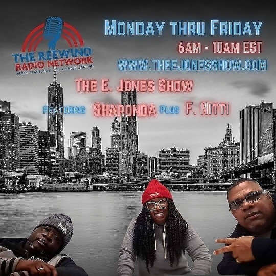
Tasty Tuesdays The E.Jones show feat Sharonda plus Nitti Dj Mark 7am wake up mix www.theejonesshow.com www.reewindradio.com #classicrnb #grownfolksmusic #liveradioshow #urbanclassics #mixtapemusic #80smusic #90smusic #wreedb #reewind 6am to 10am https://www.instagram.com/p/CPA4CiLL1CK/?utm_medium=tumblr
#classicrnb#grownfolksmusic#liveradioshow#urbanclassics#mixtapemusic#80smusic#90smusic#wreedb#reewind
0 notes
Photo

#arquitetura #arquiteturadeinteriores #cotaempreendimentos #urbanclassics (em Rua Almirante Tamandaré Itajaí Sc) https://www.instagram.com/p/CAdTUoxnrX0/?igshid=1r0sajyf4kwb7
0 notes
Photo

Big badges #britishmade #madeinengland #screenprinting #embroidery #puffembroidery #snapback #truckers #customgarments #relabelling #dtg #screenprint #fashion #yupoong #highstreet #woveninc #ukstreetwear #crossfit #urbanclassics #necklabels #ukscreenprint #northeast #cutandsew #garmentfinishing #merchandise #directtogarment #printlife #flexfit #3DEmbroidery #workwear ✉️ [email protected] ☎️ 0191 543 6966 💻 www.woveninc.com (at Woven Inc Ltd) https://www.instagram.com/p/CSYuiKvDj8g/?utm_medium=tumblr
#britishmade#madeinengland#screenprinting#embroidery#puffembroidery#snapback#truckers#customgarments#relabelling#dtg#screenprint#fashion#yupoong#highstreet#woveninc#ukstreetwear#crossfit#urbanclassics#necklabels#ukscreenprint#northeast#cutandsew#garmentfinishing#merchandise#directtogarment#printlife#flexfit#3dembroidery#workwear
1 note
·
View note
Photo

Happy Sunset ☀️ Ledersandalen für Männer kommen immer mehr in den Trend. Diese Sandale aus schwarzem Rindsleder hat eine Vollledersohle mit flachem Absatz und ist eine klassisch-elegante Variante für den Sommer. #zehaberlin #urbanclassics #mensfashion #sandalen #sandals #sandali #footwear #herrenmode #menstyle #menstreetstyle (hier: Germany) https://www.instagram.com/p/CQoob4vr2_a/?utm_medium=tumblr
#zehaberlin#urbanclassics#mensfashion#sandalen#sandals#sandali#footwear#herrenmode#menstyle#menstreetstyle
0 notes
Video
THROWBACK THURSDAY
#TBT “Crooklyn” (1994) ~ A Spike Lee Joint… Poor little Troy had no clue what she was watching here!?!? All she wanted to do was go to the bodega and get her snacks. Simple!!! Set in Brooklyn, New York, Spike and his sister Joi based the movie’s plot loosely on the story of their own lives… growing up during the early 70’s in Bed-Stuy. This is one for “The List” of all-time favorites. Two thumbs up!!! What say you??? Check the #abctbt for the title track…
#tbt#abctbt#tvshows#televisionsitcoms#sitcoms#moviequotes#movieclips#movies#classicmovies#blackmovies#cultclassics#blackhollywood#blackfilms#blacktv#urbanclassics#comedy#comedians#blackcomics#blackactors#blackcinema#bboy#hiphop#hiphopculture#hiphopfamily#spikelee#brooklyn#newyorkcity#90smovies#90shiphop
4 notes
·
View notes
Photo

Urban Classics Hooded Bubble Vest
0 notes
Photo

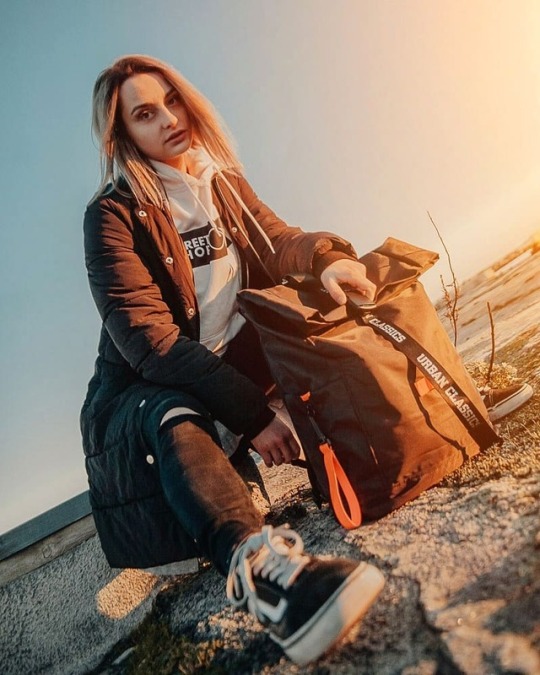
Love classics #oldschool #oldschoolcars #oldschoolfashion #urban #urbanclassic #urbanclassics #nitrobags #nitrobagsurbanclassic #fashionblogger #fashionblogger_de #fashionaddict
#oldschoolfashion#fashionblogger_de#oldschoolcars#oldschool#urbanclassics#fashionblogger#urbanclassic#nitrobagsurbanclassic#nitrobags#urban#fashionaddict
1 note
·
View note
Photo

Ganas de verano!
0 notes