#neural_network

[vladimir777sk]

👽 Эволюция за 13 секунд. Нейросеть Luma AI сгенерировало процесс развития человечества от каменного века до 5000 года. По версии нейросети НЛО — это мы из будущего.

Неожиданный поворот 🤔

Evolution in 13 seconds. The Luma AI neural network generated the process of human development from the Stone Age to the year 5000. According to the neural network, UFOs are us from the future. An unexpected twist

источник

[phonemantra-blog]

As part of Kickstarter The unusual concept of a modular mini-PC Khadas Mind has ceased to be a concept. The company has launched on Kickstarter and is ready to begin shipping some of the modules this year.  [caption id="attachment_53208" align="aligncenter" width="780"] Khadas Mind[/caption] Not much has changed since the concept was announced in July. Khadas Mind is still a very compact mini-PC that can be greatly expanded through modules. The mini-PC itself has dimensions of 146 × 105 × 20 mm with a mass of 450 g. Inside, you can choose either Core i5-1340P or Core i7-1360P, 16–32 GB of RAM, an SSD with a capacity of 512 GB, and there is also a slot for a second storage, Wi-Fi 6E, Bluetooth 5.3, USB 3.2 Gen2 (x2), HDMI 2.0, RJ45, USB-C (x2) and SD card slot. To connect those same modules, a proprietary Mind Link connector is used. It also has its own 5.55 Wh battery, which is needed for hot-swap modules.   Khadas Mind is now available for pre-order [caption id="attachment_53209" align="aligncenter" width="680"] Khadas Mind[/caption] As part of a crowdfunding campaign for a PC, they ask for 600 or 800 dollars, depending on the modification. Retail prices will be $800 and $1,100 respectively.  The base module is the Mind Dock, which expands the set of ports and adds a convenient physical volume control.   Mind Graphics is an external graphics card. This is the RTX 4060 Ti 8GB. The unit has its own set of ports and speakers. For a mini PC with a docking station, they are now asking for $ 930, and for a kit with a video card, you will have to pay at least $ 1,500.   https://youtu.be/xWjuh9XoMqo The equipment also includes the Mind xPlay module, which is a screen with a keyboard and a stand. Connecting to a mini PC turns the whole thing into a laptop. True, for some reason, there are no details about this module, and it is missing from the roadmap. It is only in the plans for now, like the Mind Studio Display monitor. 

[ladookhotnikov]

From benefits to disaster

The article notes growing concerns about the use of artificial intelligence for military purposes. This is causing excitement about the possibility of creating a new superweapon comparable in importance to nuclear weapons.  there is now a merciless race for superiority in the development of such weapons.

Another aspect that is discussed in the text is the possibility of using artificial intelligence to create autonomous weapons controlled by neural networks. This can lead to disaster if the system gets out of control.

[edujournalblogs]

Machine Learning and its applications

Machine Learning is an application of AI that provides systems the ability to automatically learn and improve from experience without being explicitly programmed. it focus on development of computer programs that can access data and use it learn for themselves.. In other words, Machine learning is all about providing data to the machine and expecting the machine to learn from the data to make its decision in the future.

The difference between the traditional programming language (like Java, C#, PHP etc) and machine language is that for traditional languages we are providing instruction to the computer in the form of coding and we are generating the output from that whereas in the case of Machine Learning, we are basically dumping a whole bunch of historical data before the system and asking it to learn by itself and generate a pattern. it will do it with specific algorithms provided by us. Here, we are providing both the input and output to the model as input to the model and provides the logic as output. For instance, in the model we can use convolutional networks for identifying complicated images such as AI camera in traffic junctions to find vehicles jumping the signals or we can use a neural networks for NLP in sentimental analysis etc.

The various implementations in machine learning are Netflix (ie., suggest various movies as per your liking), amazon customer preference, Google Maps, Telsa Self Driving Cars, Object/Face/Speech Recognition, sentimental analysis on text or speech and find out the good and bad reviews, Fraud Detectiion, Virtual Assistant like Siri and Alexa etc

Check out our master program in Data Science and ASP.NET- Complete Beginner to Advanced course and boost your confidence and knowledge.

URL: www.edujournal.com

[jobrxiv]

Postdoctoral position: Neural control of cardiorespiratory function University of Missouri A postdoctoral position is available for self-motivated researchers interested in neural control of cardiorespiratory function in health and disease See the full job description on jobRxiv: https://jobrxiv.org/job/university-of-missouri-27778-postdoctoral-position-neural-control-of-cardiorespiratory-function/?feed_id=86857 #animal_models #cardiovascular #neural_networks #optogenetics #respiratory #ScienceJobs #hiring #research

[ithisatanytime]

(onlytom)

[libarty-t]

Report №30

//-Finish mounting "Features of publishing pictures" //-Description --"In that tutorial we will study --1 How to properly publish [Image] and [Gallery]. --2 Setting up sticky notes --3 Drawing for teaching neural network.”

[kasradoc]

‏‎. سیستم های خبره : تعریف سیستم: سیستم مجموعه ای هدفدار از عناصر وروابط بین آنها است که شامل ورودی فرایند خروجی و بازخور می باشد. شروع تفکر سیستمی از سال ۱۹۶۰ وبه اوج رسیدن آن از دهه ۱۹۸۰ می باشد. ویژگیهای سیستم: سیستم ها با محیط اطراف خود در ار تباطند. سیستم ها دارای مرز نسبی هستند ومرز مطلق وجود ندارد. اجزای سیستم: داده ها مواد اولیه خروجی هر سیستم اطلاعاتی به شمار می آیند. فرایند مجموعه ای از اعمال منطقی برای تبدیل ورودی هر سیستم به خروجی آن. خروجیها (در این درس اطلاعات) شامل مواد پردازش شده مورد نیاز سازمانی که سیستم در آن قرار دارد می باشد. بازخورد (روابط کنترلی) شامل مجموعه فرامینی است که با تاثیر بر روی سه جزء دیگر منجر به رفع نقص وبهبود خروجی می شود. نکته: از مجموع روابط (Relationships) در یک سیستم ارتباطات (Communications) بوجود می آید. سیستم اطلاعات: سیستمی که برای کاربران سازمان داده یا اطلاعات فراهم م یکند که اگر در ای ن سیستم از کامپیوتر استفاده شود به آن سیستم اطلاعات مکانیزه می گویند. دانلود نمایید: http://www.kasradoc.com/product/expert-systems/ #PDF #Portable_Document_Format #Document #Kasradoc #Knowledge_Base #Inference_Engine #Explanation_Facilities #Neural_Network #Genetic_Algorithms #مقاله #پروژه #کسری_داک #سیستم_های_خبره #برنامه_نویسی_سیستم_های_خبره #جزوه_درس_سیستم_هاي_خبره #جزوه_درس_سیستمهاي_خبره #جزوه_سیستم_های_خبره #خبره #سامانه‌_های_خبره #سامانه‌_های_اطلاعاتی #مدل_سیستم_خبره #پایگاه_دانش #موتور_استنتاج #امکانات_توضیح #رابط_کاربر #مزایای_سیستم_خبره #مشخصه‌_های_سیستم_خبره #شبکه‌_های_عصبی #الگوریتم‌_های_ژنتیک #سامانه‌_های_منطق_فازی‎‏ https://www.instagram.com/p/CB23DRejwTm/?igshid=1ls11dj61gzl

[disktnk]

弊学大学院の名物授業，「エクセルでRecurrent Neural Networkを実装しよう」 pic.twitter.com/ea7pNoGfpX

— Shunsuke KITADA (@shunk031) July 12, 2017

[commentsense888]

Neural networks by HerissonMignion https://www.reddit.com/r/ProgrammerHumor/comments/du7eyp/neural_networks/?utm_source=ifttt

[phonemantra-blog]

Almost all parameters are unknown The Chinese company Loongson produces not only some of the most modern Chinese processors, but also GPUs. And its new development is designed to compete with Nvidia accelerators for AI, although they are far from the most productive and modern. [caption id="attachment_85288" align="aligncenter" width="600"] Loongson introduced LG200 AI accelerator[/caption] The accelerator (or its GPU) is called LG200. The characteristics of this solution, unfortunately, are unknown. The block diagram shows that the GPU consists of 16 small ALUs, four large ALUs, and one huge ALU or special purpose unit. Loongson introduced LG200 AI accelerator But the performance is known, albeit for the whole node: from 256 GFLOPS to 1 TFLOPS. Here, unfortunately, the details are again unknown, so it is unclear for which mode the performance is indicated, but even if it is FP64, the figure is quite modest, since modern monsters Nvidia and AMD offer 50-60 TFLOPS or more. At the same time, Loongson’s solution is a GPGPU, that is, it supports general-purpose computing. Unfortunately, there are no details here yet. Separately, we can recall that Loongson promised next year to release a video card that can compete with the Radeon RX 550 , whose performance (FP32) is just over 1.1 TFLOPS. It is possible that the LG200 will be a direct relative of this adapter.

[ladookhotnikov]

AI To Sack Highly Skilled Specialists

In the situations where a non-standard approach to problems solving is required, the speed of perception or the ability to structure information, AI is already superior to humans.

Mankind expected a robot implementation first in the field of physical labor. However, it seems that professions such as cleaners, farmers or cooking helpers will be with us for a long time to come.

According to a report published by the OECD, the greatest threat of extinction lies with the "white collars": managers, executives, specialists in various fields. Neural networks collect information better and faster, process it and make decisions. In fact, it is now possible to reduce entire analytical departments and implement AI without compromising the company's operation.

At the same time it is especially noted that the conclusions were made before the advent of neural networks such as ChatGPT. There is no doubt that, given these language patterns, the threat to white-collar workers is substantially increased.

On the other hand, it is concluded that not everything is so simple since AI not only reduces jobs, but also generates the creation of new ones. So not everything is so scary, white-collar workers are unlikely to face mass unemployment.

#Robotics #Artificial_Intelligence #Neural_networks #ChatGPT #Unemployment #Technology #Innovation

[edujournalblogs]

An introduction to Computer Vision

Computer Vision with deep learning is another advanced technique that employs neural networks to process and analyze visual data, such as images and videos. With deep learning, Computer Vision has become more accurate and sophisticated, enabling machines to perform highly accurate tasks such as object detection, image recognition, facial recognition, and scene segmentation. CNNs are the most commonly used deep learning models in Computer Vision because they can extract features from images and learn spatial relationships between objects.

Computer Vision applications based on deep learning have numerous practical applications in various industries, including healthcare, automotive, retail, and security. Some examples include self-driving cars, medical image analysis, surveillance systems, and augmented reality. The advancements in deep learning have enabled machines to understand the world through visual data, making computer vision an essential component in developing intelligent systems.

Check out our master program in Data Science and ASP.NET- Complete Beginner to Advanced course and boost your confidence and knowledge.

URL: www.edujournal.com

[jobrxiv]

Postdoctoral position: Neural control of cardiorespiratory function University of Missouri A postdoctoral position is available for self-motivated researchers interested in neural control of cardiorespiratory function in health and disease See the full job description on jobRxiv: https://jobrxiv.org/job/university-of-missouri-27778-postdoctoral-position-neural-control-of-cardiorespiratory-function/?feed_id=81826 #animal_models #cardiovascular #neural_networks #optogenetics #respiratory #ScienceJobs #hiring #research

[kaygun]

Feed-forward and back-propagation in neural networks as left- and right-fold

Description of the problem:

Today's post is about something (trivial) I realized a few days ago: one can reconceptualize feed-forward and back-propagation operations in a neural network as instances of left-fold and right-fold operations.  Most of this post will be theoretical, and at the end, I will write some code in scala.

Feed-forward and Back-propagation in a Neural Network

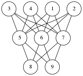
A neural network is composed of perceptrons connected via a computation graph.

A perceptron on the other hand is a computation unit which takes a vector $\mathbf{x}$ as an input and produces a scalar output

$$ f(\mathbf{w}\cdot\mathbf{x} + b) $$

Here $f$ is a function of type signature $f\colon\mathbb{R}\to \mathbb{R}$ and $\mathbf{w}$ and $b$ are parameters of the underlying perceptron.

In the simplest version of the neural networks, the network consists of layers of perceptrons where input propagates from one layer to the next. Then depending on the error produced, we back-propagate the error adjusting the weights of the perceptrons to produce the correct output. I wrote about perceptrons and back-propagation before (here, here and here)

The observation I made is this feed-forward is a left fold, while back-propagation is a right-fold operation. In pseudo-code we can express these operations as follows:

FeedForward(xs,nss) Input: a vector xs, and a list of layers nss where a layer is an ordered list of perceptron and each perceptron is a quintuple (w,b,f,eta,ys) where w is a vector, b is a real number, f is and activation function, eta is the learning rate of the perceptron and zs is the last input processed by the node. Output: a vector ys Begin If nss is empty Return xs Else Let ns <- head of nss Let ys <- () For each node=(w,f,b,zs) in ns Update zs <- xs Append f(<w,xs> + b) to ys End Call FeedForward(ys, tail of nss) End End BackPropagations(ds,nss) Input: a vector of errors, and a list of layers as before. Output: a vector Begin If nss is empty Return ds Else Let ns <- tail of nss Let zsum <- 0 For each ((w,b,f,eta,xs),d) in (ns,ds) Let zs <- (eta * d / f'(<w,xs> + b)) * xs Update w <- w - zs Update zsum <- zsum + zs End Call BackPropagation(zsum, all but the last element of nss) End End

A Scala Implementation

You can download the code and run it from my github repository. I am using mill instead of sbt.

The feed-forward part of the algorithm is easy to implement in the functional style, i.e. no mutable persistent state, such that the network as a computation unit is referentially transparent. However, the back-propagation phase requires that we update the weights of each perceptron. This means we must capture the whole state of the neural network in a data structure and propagate it along each step. As much as I like functional style and referential transparency, it is easier and cleaner to implement neural networks with mutable persistent state. Hence the choices of vars below.

package perceptron import breeze.linalg._ object neural { case class node(size: Int, fn: Double=>Double, eta: Double) { private var input = DenseVector.rand[Double](size+1) private var calc = 0.0 var weights = DenseVector.rand[Double](size+1) def forward(x: Array[Double]): Double = { input = DenseVector(Array(1.0) ++ x) calc = fn(weights.dot(input)) calc } def backprop(delta: Double): DenseVector[Double] = { val ider = eta/(fn(calc + eta/2) - fn(calc - eta/2) + eta*Math.random) val res = (-delta*eta*ider)*input weights += res res } } case class layer(size: Int, num: Int, fn: Double=>Double, eta: Double) { val nodes = (1 to num).map(i=>node(size,fn,eta)).toArray def forward(xs: Array[Double]) = nodes.map(_.forward(xs)) def backprop(ds: Array[Double]) = { val zero = DenseVector.zeros[Double](nodes(0).size+1) (nodes,ds).zipped .foldRight(zero)({ case((n,d),v) => v + n.backprop(d) }) .toArray } } case class network(shape:Array[(Int, Int, Double=>Double, Double)]) { val layers = shape.map({ case (n,m,fn,eta) => layer(n,m,fn,eta) }) def forward(xs:Array[Double]) = layers.foldLeft(xs)((ys,ns) => ns.forward(ys)) def backprop(ds:Array[Double]) = layers.foldRight(ds)((ns,ys) => ns.backprop(ys)) } } `

The only additional external dependency is the breeze math and statistics package. As for the utility code that we need for training and testing a neural network model for a given dataset, we have

package perceptron import perceptron.neural._ object Main { import scala.util.Random.nextInt import scala.io.Source.fromFile def sigmoid(x:Double) = 1.0/(1.0 + math.exp(-x)) def relu(x:Double) = math.max(x,0.0) def train(net:network, xs: Array[Array[Double]], ys: Array[Double], epochs: Int, batchSize: Int, tol: Double):Array[Double] = { val size = xs.length var err = Array[Double]() for(i <- 1 to epochs) { val j = math.abs(nextInt)%size val x = xs(j) val d = net.forward(x)(0) - ys(j) net.backprop(Array(d)) if(i % batchSize == 1) err = Array(0.0) ++ err if(math.abs(d)>tol) err(0) += 1.0/batchSize } return(err.reverse) } def main(args: Array[String]) { val file = fromFile(args(0)) val size = args(1).toInt val eta = args(2).toDouble val epochs = args(3).toInt val batchSize = args(4).toInt val tol = args(5).toDouble val data = file.mkString .split("\n") .map(x=>x.split("\t").map(_.toDouble).reverse) val ys = data.map(_.head) val xs = data.map(_.tail) val net = network(Array((size,4,relu,eta),(4,1,sigmoid,eta))) val err = train(net, xs, ys, epochs, batchSize, tol) err.foreach(x=>println("%4.3f".format(x))) } }

I know that MNIST is the de facto standard, but it is PIA to load and process the data. Instead, I am going to use the sonar dataset from UCI

I ran the model with the following parameters:

mill perceptron.run data/sonar.csv 60 0.0125 1750000 500 0.3

In the code above, the neural network has two layers: 60 nodes on the input layer, 1 hidden layer with 4 nodes, and a single output node. The perceptrons on the input layer use RELU meanwhile the other layer uses the sigmoid function.

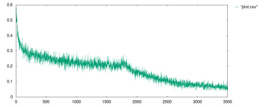
The best result I received is in the file data/plot.csv whose plot is given in

[marialaura-diazpena]

My Programming Journey: Understanding Music Genres with Machine Learning

Artificial Intelligence is used everyday, by regular people and businesses, creating such a positive impact in all kinds of industries and fields that it makes me think that AI is only here to stay and grow, and help society grow with it. AI has evolved considerably in the last decade, currently being able to do things that seem taken out of a Sci-Fi movie, like driving cars, recognizing faces and words (written and spoken), and music genres.

While Music is definitely not the most profitable application of Machine Learning, it has benefited tremendously from Deep Learning and other ML applications. The potential AI possess in the music industry includes automating services and discovering insights and patterns to classify and/or recommend music.

We can be witnesses to this potential when we go to our preferred music streaming service (such as Spotify or Apple Music) and, based on the songs we listen to or the ones we’ve previously saved, we are given playlists of similar songs that we might also like.

Machine Learning’s ability of recognition isn’t just limited to faces or words, but it can also recognize instruments used in music. Music source separation is also a thing, where a song is taken and its original signals are separated from a mixture audio signal. We can also call this Feature Extraction and it is popularly used nowadays to aid throughout the cycle of music from composition and recording to production. All of this is doable thanks to a subfield of Music Machine Learning: Music Information Retrieval (MIR). MIR is needed for almost all applications related to Music Machine Learning. We’ll dive a bit deeper on this subfield.

Music Information Retrieval

Music Information Retrieval (MIR) is an interdisciplinary field of Computer Science, Musicology, Statistics, Signal Processing, among others; the information within music is not as simple as it looks like. MIR is used to categorize, manipulate and even create music. This is done by audio analysis, which includes pitch detection, instrument identification and extraction of harmonic, rhythmic and/or melodic information. Plain information can be easily comprehended (such as tempo (beats per minute), melody, timbre, etc.) and easily calculated through different genres. However, many music concepts considered by humans can’t be perfectly modeled to this day, given there are many factors outside music that play a role in its perception.

Getting Started

I wanted to try something more of a challenge for this post, so I am attempting to Visualize and Classify audio data using the famous GTZAN Dataset to perform an in depth analysis of sound and understand what features we can visualize/extract from this kind of data. This dataset consists of: · A collection of 10 genres with 100 audio (WAV) files each, each having a length of 30 seconds. This collection is stored in a folder called “genres_original”. · A visual representation for each audio file stored in a folder called “images_original”. The audio files were converted to Mel Spectrograms (later explained) to make them able to be classified through neural networks, which take in image representation. · 2 CVS files that contain features of the audio files. One file has a mean and variance computed over multiple features for each song (full length of 30 seconds). The second CVS file contains the same songs but split before into 3 seconds, multiplying the data times 10. For this project, I am yet again coding in Visual Studio Code. On my last project I used the Command Line from Anaconda (which is basically the same one from Windows with the python environment set up), however, for this project I need to visualize audio data and these representations can’t be done in CLI, so I will be running my code from Jupyter Lab, from Anaconda Navigator. Jupyter Lab is a web-based interactive development environment for Jupyter notebooks (documents that combine live runnable code with narrative text, equations, images and other interactive visualizations). If you haven’t installed Anaconda Navigator already, you can find the installation steps on my previous blog post. I would quickly like to mention that Tumblr has a limit of 10 images per post, and this is a lengthy project so I’ll paste the code here instead of uploading code screenshots, and only post the images of the outputs. The libraries we will be using are:

> pandas: a data analysis and manipulation library.

> numpy: to work with arrays.

> seaborn: to visualize statistical data based on matplolib.

> matplotlib.pyplot: a collection of functions to create static, animated and interactive visualizations.

> Sklearn: provides various tools for model fitting, data preprocessing, model selection and evaluation, among others.

· naive_bayes

· linear_model

· neighbors

· tree

· ensemble

· svm

· neural_network

· metrics

· preprocessing

· decomposition

· model_selection

· feature_selection

> librosa: for music and audio analysis to create MIR systems.

· display

> IPython: interactive Python

· display import Audio

> os: module to provide functions for interacting with the operating system.

> xgboost: gradient boosting library

· XGBClassifier, XGBRFClassifier

· plot_tree, plot_importance

> tensorflow:

· Keras

· Sequential and layers

Exploring Audio Data

Sounds are pressure waves, which can be represented by numbers over a time period. We first need to understand our audio data to see how it looks. Let’s begin with importing the libraries and loading the data:

import pandas as pd

import numpy as np

import seaborn as sns

import matplotlib.pyplot as plt

import sklearn

import librosa

import librosa.display

import IPython.display as ipd

from IPython.display import Audio

import os

from sklearn.naive_bayes import GaussianNB

from sklearn.linear_model import SGDClassifier, LogisticRegression

from sklearn.neighbors import KNeighborsClassifier

from sklearn.tree import DecisionTreeClassifier

from sklearn.ensemble import RandomForestClassifier

from sklearn.svm import SVC

from sklearn.neural_network import MLPClassifier

from xgboost import XGBClassifier, XGBRFClassifier

from xgboost import plot_tree, plot_importance

from sklearn.metrics import confusion_matrix, accuracy_score, roc_auc_score, roc_curve

from sklearn import preprocessing

from sklearn.decomposition import PCA

from sklearn.model_selection import train_test_split

from sklearn.feature_selection import RFE

from tensorflow.keras import Sequential

from tensorflow.keras.layers import *

import warnings

warnings.filterwarnings('ignore')

# Loading the data

general_path = 'C:/Users/807930/Documents/Spring 2021/Emerging Trends in Technology/MusicGenre/input/gtzan-database-music-genre-classification/Data'

Now let’s load one of the files (I chose Hit Me Baby One More Time by Britney Spears):

print(list(os.listdir(f'{general_path}/genres_original/')))

#Importing 1 file to explore how our Audio Data looks.

y, sr = librosa.load(f'{general_path}/genres_original/pop/pop.00019.wav')

#Playing the audio

ipd.display(ipd.Audio(y, rate=sr, autoplay=True))

print('Sound (Sequence of vibrations):', y, '\n')

print('Sound shape:', np.shape(y), '\n')

print('Sample Rate (KHz):', sr, '\n')

# Verify length of the audio

print('Check Length of Audio:', 661794/22050)

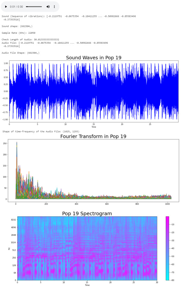
We took the song and using the load function from the librosa library, we got an array of the audio time series (sound) and the sample rate of sound. The length of the audio is 30 seconds. Now we can trim our audio to remove the silence between songs and use the librosa.display.waveplot function to plot the audio file into a waveform. > Waveform: The waveform of an audio signal is the shape of its graph as a function of time.

# Trim silence before and after the actual audio

audio_file, _ = librosa.effects.trim(y)

print('Audio File:', audio_file, '\n')

print('Audio File Shape:', np.shape(audio_file))

#Sound Waves 2D Representation

plt.figure(figsize = (16, 6))

librosa.display.waveplot(y = audio_file, sr = sr, color = "b");

plt.title("Sound Waves in Pop 19", fontsize = 25);

After having represented the audio visually, we will plot a Fourier Transform (D) from the frequencies and amplitudes of the audio data. > Fourier Transform: A mathematical function that maps the frequency and phase content of local sections of a signal as it changes over time. This means that it takes a time-based pattern (in this case, a waveform) and retrieves the complex valued function of frequency, as a sine wave. The signal is converted into individual spectral components and provides frequency information about the signal.

#Default Fast Fourier Transforms (FFT)

n_fft = 2048 # window size

hop_length = 512 # number audio of frames between STFT columns

# Short-time Fourier transform (STFT)

D = np.abs(librosa.stft(audio_file, n_fft = n_fft, hop_length = hop_length))

print('Shape of time-frequency of the Audio File:', np.shape(D))

plt.figure(figsize = (16, 6))

plt.plot(D);

plt.title("Fourier Transform in Pop 19", fontsize = 25);

The Fourier Transform only gives us information about the frequency values and now we need a visual representation of the frequencies of the audio signal so we can calculate more audio features for our system. To do this we will plot the previous Fourier Transform (D) into a Spectrogram (DB). > Spectrogram: A visual representation of the spectrum of frequencies of a signal as it varies with time.

DB = librosa.amplitude_to_db(D, ref = np.max)

# Creating the Spectrogram

plt.figure(figsize = (16, 6))

librosa.display.specshow(DB, sr = sr, hop_length = hop_length, x_axis = 'time', y_axis = 'log'

cmap = 'cool')

plt.colorbar();

plt.title("Pop 19 Spectrogram", fontsize = 25);

The output:

Audio Features

Now that we know what the audio data looks like to python, we can proceed to extract the Audio Features. The features we will need to extract, based on the provided CSV, are: · Harmonics · Percussion · Zero Crossing Rate · Tempo · Spectral Centroid · Spectral Rollof · Mel-Frequency Cepstral Coefficients · Chroma Frequencies Let’s start with the Harmonics and Percussive components:

# Decompose the Harmonics and Percussive components and show Representation

y_harm, y_perc = librosa.effects.hpss(audio_file)

plt.figure(figsize = (16, 6))

plt.plot(y_harm, color = 'g');

plt.plot(y_perc, color = 'm');

plt.title("Harmonics and Percussive components", fontsize = 25);

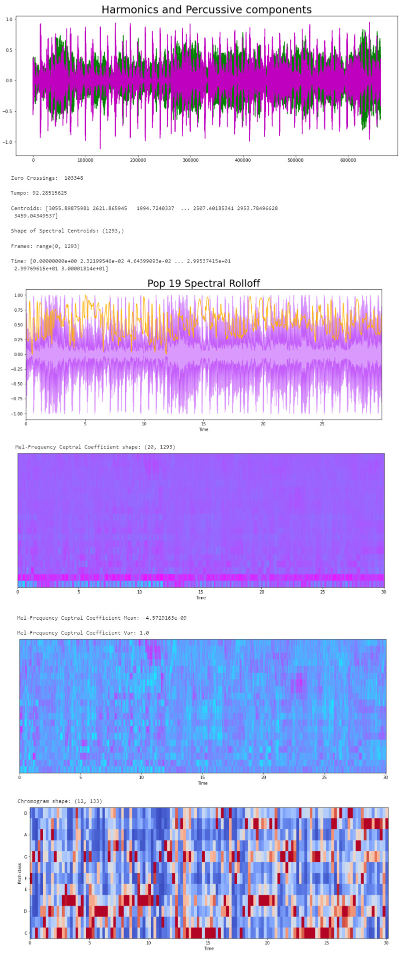
Using the librosa.effects.hpss function, we are able to separate the harmonics and percussive elements from the audio source and plot it into a visual representation.

Now we can retrieve the Zero Crossing Rate, using the librosa.zero_crossings function.

> Zero Crossing Rate: The rate of sign-changes (the number of times the signal changes value) of the audio signal during the frame.

#Total number of zero crossings

zero_crossings = librosa.zero_crossings(audio_file, pad=False)

print(sum(zero_crossings))

The Tempo (Beats per Minute) can be retrieved using the librosa.beat.beat_track function.

# Retrieving the Tempo in Pop 19

tempo, _ = librosa.beat.beat_track(y, sr = sr)

print('Tempo:', tempo , '\n')

The next feature extracted is the Spectral Centroids. > Spectral Centroid: a measure used in digital signal processing to characterize a spectrum. It determines the frequency area around which most of the signal energy concentrates.

# Calculate the Spectral Centroids

spectral_centroids = librosa.feature.spectral_centroid(audio_file, sr=sr)[0]

print('Centroids:', spectral_centroids, '\n')

print('Shape of Spectral Centroids:', spectral_centroids.shape, '\n')

# Computing the time variable for visualization

frames = range(len(spectral_centroids))

# Converts frame counts to time (seconds)

t = librosa.frames_to_time(frames)

print('Frames:', frames, '\n')

print('Time:', t)

Now that we have the shape of the spectral centroids as an array and the time variable (from frame counts), we need to create a function that normalizes the data. Normalization is a technique used to adjust the volume of audio files to a standard level which allows the file to be processed clearly. Once it’s normalized we proceed to retrieve the Spectral Rolloff.

> Spectral Rolloff: the frequency under which the cutoff of the total energy of the spectrum is contained, used to distinguish between sounds. The measure of the shape of the signal.

# Function that normalizes the Sound Data

def normalize(x, axis=0):

return sklearn.preprocessing.minmax_scale(x, axis=axis)

# Spectral RollOff Vector

spectral_rolloff = librosa.feature.spectral_rolloff(audio_file, sr=sr)[0]

plt.figure(figsize = (16, 6))

librosa.display.waveplot(audio_file, sr=sr, alpha=0.4, color = '#A300F9');

plt.plot(t, normalize(spectral_rolloff), color='#FFB100');

Using the audio file, we can continue to get the Mel-Frequency Cepstral Coefficients, which are a set of 20 features. In Music Information Retrieval, it’s often used to describe timbre. We will employ the librosa.feature.mfcc function.

mfccs = librosa.feature.mfcc(audio_file, sr=sr)

print('Mel-Frequency Ceptral Coefficient shape:', mfccs.shape)

#Displaying the Mel-Frequency Cepstral Coefficients:

plt.figure(figsize = (16, 6))

librosa.display.specshow(mfccs, sr=sr, x_axis='time', cmap = 'cool');

The MFCC shape is (20, 1,293), which means that the librosa.feature.mfcc function computed 20 coefficients over 1,293 frames.

mfccs = sklearn.preprocessing.scale(mfccs, axis=1)

print('Mean:', mfccs.mean(), '\n')

print('Var:', mfccs.var())

plt.figure(figsize = (16, 6))

librosa.display.specshow(mfccs, sr=sr, x_axis='time', cmap = 'cool');

Now we retrieve the Chroma Frequencies, using librosa.feature.chroma_stft. > Chroma Frequencies (or Features): are a powerful tool for analyzing music by categorizing pitches. These features capture harmonic and melodic characteristics of music.

# Increase or decrease hop_length to change how granular you want your data to be

hop_length = 5000

# Chromogram

chromagram = librosa.feature.chroma_stft(audio_file, sr=sr, hop_length=hop_length)

print('Chromogram shape:', chromagram.shape)

plt.figure(figsize=(16, 6))

librosa.display.specshow(chromagram, x_axis='time', y_axis='chroma', hop_length=hop_length, cmap='coolwarm');

The output:

Exploratory Data Analysis

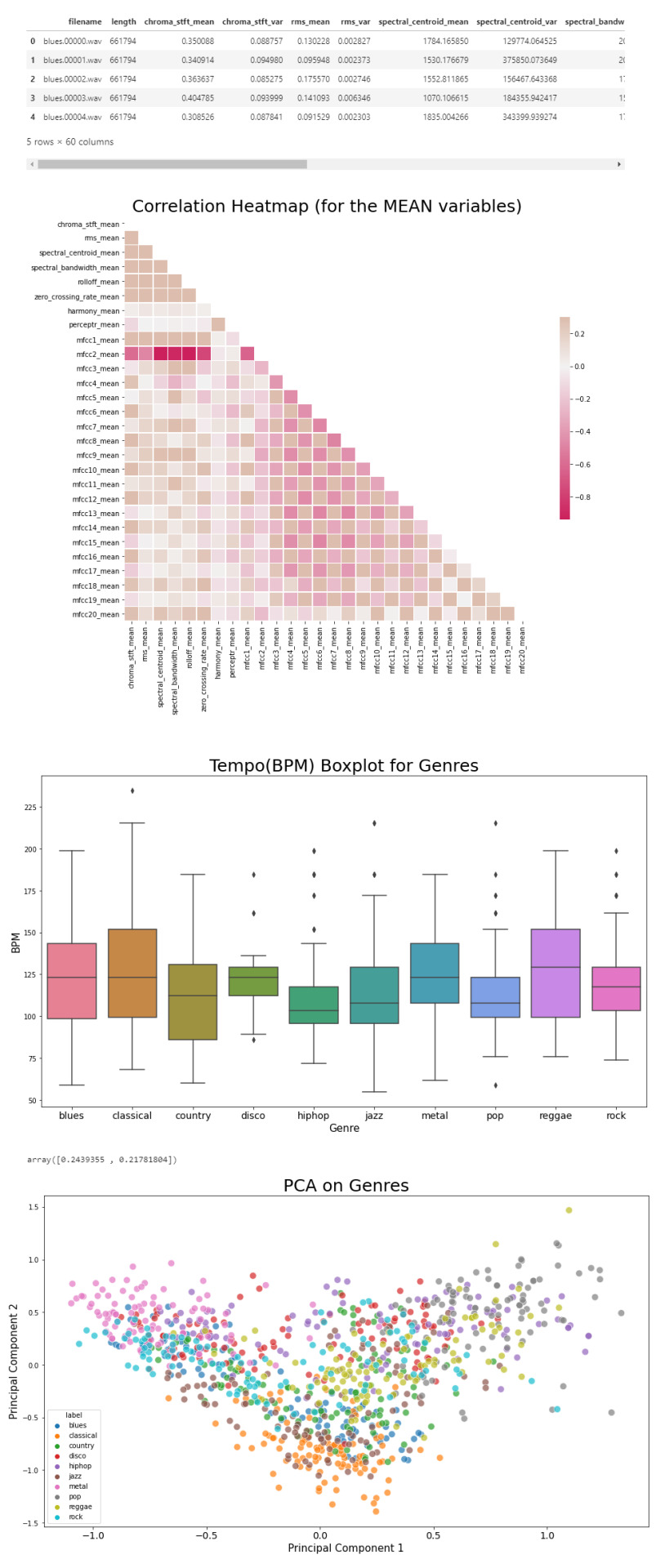
Now that we have a visual understanding of what an audio file looks like, and we’ve explored a good set of features, we can perform EDA, or Exploratory Data Analysis. This is all about getting to know the data and data profiling, summarizing the dataset through descriptive statistics. We can do this by getting a description of the data, using the describe() function or head() function. The describe() function will give us a description of all the dataset rows, and the head() function will give us the written data. We will perform EDA on the csv file, which contains all of the features previously analyzed above, and use the head() function:

# Loading the CSV file

data = pd.read_csv(f'{general_path}/features_30_sec.csv')

data.head()

Now we can create the correlation matrix of the data found in the csv file, using the feature means (average). We do this to summarize our data and pass it into a Correlation Heatmap.

# Computing the Correlation Matrix

spike_cols = [col for col in data.columns if 'mean' in col]

corr = data[spike_cols].corr()

The corr() function finds a pairwise correlation of all columns, excluding non-numeric and null values.

Now we can plot the heatmap:

# Generate a mask for the upper triangle

mask = np.triu(np.ones_like(corr, dtype=np.bool))

# Set up the matplotlib figure

f, ax = plt.subplots(figsize=(16, 11));

# Generate a custom diverging colormap

cmap = sns.diverging_palette(0, 25, as_cmap=True, s = 90, l = 45, n = 5)

# Draw the heatmap with the mask and correct aspect ratio

sns.heatmap(corr, mask=mask, cmap=cmap, vmax=.3, center=0,

square=True, linewidths=.5, cbar_kws={"shrink": .5}

plt.title('Correlation Heatmap (for the MEAN variables)', fontsize = 25)

plt.xticks(fontsize = 10)

plt.yticks(fontsize = 10);

Now we will take the data and, extracting the label(genre) and the tempo, we will draw a Box Plot. Box Plots visually show the distribution of numerical data through displaying percentiles and averages.

# Setting the axis for the box plot

x = data[["label", "tempo"]]

f, ax = plt.subplots(figsize=(16, 9));

sns.boxplot(x = "label", y = "tempo", data = x, palette = 'husl');

plt.title('Tempo(BPM) Boxplot for Genres', fontsize = 25)

plt.xticks(fontsize = 14)

plt.yticks(fontsize = 10);

plt.xlabel("Genre", fontsize = 15)

plt.ylabel("BPM", fontsize = 15)

Now we will draw a Scatter Diagram. To do this, we need to visualize possible groups of genres:

# To visualize possible groups of genres

data = data.iloc[0:, 1:]

y = data['label']

X = data.loc[:, data.columns != 'label']

We use data.iloc to get rows and columns at integer locations, and data.loc to get rows and columns with particular labels, excluding the label column. The next step is to normalize our data:

# Normalization

cols = X.columns

min_max_scaler = preprocessing.MinMaxScaler()

np_scaled = min_max_scaler.fit_transform(X)

X = pd.DataFrame(np_scaled, columns = cols)

Using the preprocessing library, we rescale each feature to a given range. Then we add a fit to data and transform (fit_transform).

We can proceed with a Principal Component Analysis:

# Principal Component Analysis

pca = PCA(n_components=2)

principalComponents = pca.fit_transform(X)

principalDf = pd.DataFrame(data = principalComponents, columns = ['principal component 1', 'principal component 2'])

# concatenate with target label

finalDf = pd.concat([principalDf, y], axis = 1)

PCA is used to reduce dimensionality in data. The fit learns some quantities from the data. Before the fit transform, the data shape was [1000, 58], meaning there’s 1000 rows with 58 columns (in the CSV file there’s 60 columns but two of these are string values, so it leaves with 58 numeric columns).

Once we use the PCA function, and set the components number to 2 we reduce the dimension of our project from 58 to 2. We have found the optimal stretch and rotation in our 58-dimension space to see the layout in two dimensions.

After reducing the dimensional space, we lose some variance(information).

pca.explained_variance_ratio_

By using this attribute we get the explained variance ratio, which we sum to get the percentage. In this case the variance explained is 46.53% .

plt.figure(figsize = (16, 9))

sns.scatterplot(x = "principal component 1", y = "principal component 2", data = finalDf, hue = "label", alpha = 0.7,

s = 100);

plt.title('PCA on Genres', fontsize = 25)

plt.xticks(fontsize = 14)

plt.yticks(fontsize = 10);

plt.xlabel("Principal Component 1", fontsize = 15)

plt.ylabel("Principal Component 2", fontsize = 15)

plt.savefig("PCA Scattert.jpg")

The output:

Genre Classification

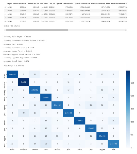
Now we know what our data looks like, the features it has and have analyzed the principal component on all genres. All we have left to do is to build a classifier model that will predict any new audio data input its genre. We will use the CSV with 10 times the data for this.

# Load the data

data = pd.read_csv(f'{general_path}/features_3_sec.csv')

data = data.iloc[0:, 1:]

data.head()

Once again visualizing and normalizing the data.

y = data['label'] # genre variable.

X = data.loc[:, data.columns != 'label'] #select all columns but not the labels

# Normalization

cols = X.columns

min_max_scaler = preprocessing.MinMaxScaler()

np_scaled = min_max_scaler.fit_transform(X)

# new data frame with the new scaled data.

X = pd.DataFrame(np_scaled, columns = cols)

Now we have to split the data for training. Like I did in my previous post, the proportions are (70:30). 70% of the data will be used for training and 30% of the data will be used for testing.

# Split the data for training

X_train, X_test, y_train, y_test = train_test_split(X, y, test_size=0.3, random_state=42)

I tested 7 algorithms but I decided to go with K Nearest-Neighbors because I had previously used it.

knn = KNeighborsClassifier(n_neighbors=19)

knn.fit(X_train, y_train)

preds = knn.predict(X_test)

print('Accuracy', ':', round(accuracy_score(y_test, preds), 5), '\n')

# Confusion Matrix

confusion_matr = confusion_matrix(y_test, preds) #normalize = 'true'

plt.figure(figsize = (16, 9))

sns.heatmap(confusion_matr, cmap="Blues", annot=True,

xticklabels = ["blues", "classical", "country", "disco", "hiphop", "jazz", "metal", "pop", "reggae", "rock"],

yticklabels=["blues", "classical", "country", "disco", "hiphop", "jazz", "metal", "pop", "reggae", "rock"]);

The output:

References

· https://medium.com/@james_52456/machine-learning-and-the-future-of-music-an-era-of-ml-artists-9be5ef27b83e

· https://www.kaggle.com/andradaolteanu/work-w-audio-data-visualise-classify-recommend/

· https://www.kaggle.com/dapy15/music-genre-classification/notebook

· https://towardsdatascience.com/how-to-start-implementing-machine-learning-to-music-4bd2edccce1f

· https://en.wikipedia.org/wiki/Music_information_retrieval

· https://pandas.pydata.org

· https://scikit-learn.org/

· https://seaborn.pydata.org

· https://matplotlib.org

· https://librosa.org/doc/main/index.html

· https://github.com/dmlc/xgboost

· https://docs.python.org/3/library/os.html

· https://www.tensorflow.org/

· https://www.hindawi.com/journals/sp/2021/1651560/