#dataimportant

[walkboss1]

python programming company

A high-level, all-purpose programming language is Python. Code readability is prioritised in its design philosophy, which makes heavy use of indentation. Python uses garbage collection and has dynamic typing. It supports a variety of programming paradigms, such as functional, object-oriented, and structured programming. Nowadays, a lot of Linux and UNIX distributions offer a modern Python, and installing Python is typically simple. Even some Windows machines now come pre-installed with Python, most notably those made by HP. For most platforms, installing Python is straightforward, but if you do need to do so and are unsure how to go about it, you can find some tips on the Beginners Guide/Download wiki page.

[spiritsofts]

Learn expert level Online EPBCS Training in our best institute real time Oracle EPBCS (Enterprise Planning and Budgeting Cloud Services) Certification Training with Course Material Pdf attend demo free Live Oracle EPBCS Tutorial Videos for Beginners and Download Oracle EPBCS Documentation Dumps Within Reasonable Cost in Hyderabad Bangalore Mumbai Delhi India UAE USA Canada Toronto Texas California Australia Singapore Malaysia South Africa Brazil Spain Japan China UK Germany London England Dubai Qatar Oman Mexico France Srilanka Pune Noida Chennai Pakistan

https://www.spiritsofts.com/oracle-epbcs-online-training/

Enhance Financial Control with Oracle ARCS Online Training

Cloud-Based Reconciliation: Oracle ARCS training focuses on utilizing cloud technology to enhance reconciliation efficiency and accuracy, allowing participants to manage reconciliations from anywhere.

End-to-End Process: The training covers the entire reconciliation lifecycle, from data import and matching to review, approval, and reporting, ensuring participants grasp the complete process flow.

Data Integrity and Validation: Learners gain insights into data validation techniques, ensuring data integrity before initiating the reconciliation process, minimizing errors, and improving reliability.

Automated Matching: The training emphasizes leveraging automation to match large volumes of data, reducing manual efforts, and expediting the reconciliation process.

[teguhteja]

Mastering Odoo: From Barcode Validation to Advanced Data Imports

#Odoo #DataImport #BarcodeValidation Unlock Odoo's potential! Our latest blog post guides you through barcode validation, efficient data imports, and understanding Odoo's data models. Perfect for businesses looking to streamline their processes and maximi

Ensuring Accurate Barcodes in Odoo Odoo data imports and barcode validation. Barcodes play a crucial role in inventory management. Let’s explore how to validate barcodes, specifically the EN13 pattern, in Odoo. Implementing EN13 Barcode Validation To validate EN13 barcodes, we need to check both the length and the check digit. Here’s a simple Python code snippet to get you started: def…

[coursera2022]

Logistic Regression

Assignment: Test a Logistic Regression Model

Following is the Python program I wrote to fulfill the fourth assignment of the Regression Modeling in Practice online course.

I decided to use Jupyter Notebook as it is a pretty way to write code and present results.

Research question for this assignment

For this assignment, I decided to use the NESARC database with the following question : Are people from white ethnicity more likely to have ever used cannabis?

The potential other explanatory variables will be:

Age

Sex

Family income

Data management

The data will be managed to get cannabis usage recoded from 0 (never used cannabis) and 1 (used cannabis). The non-answering recordings (reported as 9) will be discarded.

The response variable having 2 categories, categories grouping is not needed.

The other categorical variable (sex) will be recoded such that 0 means female and 1 equals male. And the two quantitative explanatory variables (age and family income) will be centered.

In [1]:# Magic command to insert the graph directly in the notebook%matplotlib inline # Load a useful Python libraries for handling dataimport pandas as pd import numpy as np import statsmodels.formula.api as smf import seaborn as sns import matplotlib.pyplot as plt from IPython.display import Markdown, display

In [2]:nesarc = pd.read_csv('nesarc_pds.csv') C:\Anaconda3\lib\site-packages\IPython\core\interactiveshell.py:2723: DtypeWarning: Columns (76) have mixed types. Specify dtype option on import or set low_memory=False. interactivity=interactivity, compiler=compiler, result=result)

In [3]:canabis_usage = {1 : 1, 2 : 0, 9 : 9} sex_shift = {1 : 1, 2 : 0} white_race = {1 : 1, 2 : 0} subnesarc = (nesarc[['AGE', 'SEX', 'S1Q1D5', 'S1Q7D', 'S3BQ1A5', 'S1Q11A']] .assign(sex=lambda x: pd.to_numeric(x['SEX'].map(sex_shift)), white_ethnicity=lambda x: pd.to_numeric(x['S1Q1D5'].map(white_race)), used_canabis=lambda x: (pd.to_numeric(x['S3BQ1A5'], errors='coerce') .map(canabis_usage) .replace(9, np.nan)), family_income=lambda x: (pd.to_numeric(x['S1Q11A'], errors='coerce'))) .dropna()) centered_nesarc = subnesarc.assign(age_c=subnesarc['AGE']-subnesarc['AGE'].mean(), family_income_c=subnesarc['family_income']-subnesarc['family_income'].mean())

In [4]:display(Markdown("Mean age : {:.0f}".format(centered_nesarc['AGE'].mean()))) display(Markdown("Mean family income last year: {:.0f}$".format(centered_nesarc['family_income'].mean())))

Mean age : 46

Mean family income last year: 45631$

Let's check that the quantitative variable are effectively centered.

In [5]:print("Centered age") print(centered_nesarc['age_c'].describe()) print("\nCentered family income") print(centered_nesarc['family_income_c'].describe()) Centered age count 4.272500e+04 mean -2.667486e-13 std 1.819181e+01 min -2.841439e+01 25% -1.441439e+01 50% -2.414394e+00 75% 1.258561e+01 max 5.158561e+01 Name: age_c, dtype: float64 Centered family income count 4.272500e+04 mean -5.710829e-10 std 5.777221e+04 min -4.560694e+04 25% -2.863094e+04 50% -1.263094e+04 75% 1.436906e+04 max 2.954369e+06 Name: family_income_c, dtype: float64

The means are both very close to 0; confirming the centering.

Distributions visualization

The following plots shows the distribution of all 3 explanatory variables with the response variable.

In [6]:g = sns.factorplot(x='white_ethnicity', y='used_canabis', data=centered_nesarc, kind="bar", ci=None) g.set_xticklabels(['Non White', 'White']) plt.xlabel('White ethnicity') plt.ylabel('Ever used cannabis') plt.title('Ever used cannabis dependance on the white ethnicity');

In [7]:g = sns.factorplot(x='sex', y='used_canabis', data=centered_nesarc, kind="bar", ci=None) g.set_xticklabels(['Female', 'Male']) plt.ylabel('Ever used cannabis') plt.title('Ever used cannabis dependance on the sex');

In [8]:g = sns.boxplot(x='used_canabis', y='family_income', data=centered_nesarc) g.set_yscale('log') g.set_xticklabels(('No', 'Yes')) plt.xlabel('Ever used cannabis') plt.ylabel('Family income ($)');

In [9]:g = sns.boxplot(x='used_canabis', y='AGE', data=centered_nesarc) g.set_xticklabels(('No', 'Yes')) plt.xlabel('Ever used cannabis') plt.ylabel('Age');

The four plots above show the following trends:

More white people tries cannabis more than non-white

Male people tries cannabis more than female

Younger people tries cannabis more than older ones

Man from richer families tries cannabis more than those from poorer families

Logistic regression model

The plots showed the direction of a potential relationship. But a rigorous statistical test has to be carried out to confirm the four previous hypothesis.

The following code will test a logistic regression model on our hypothesis.

In [10]:model = smf.logit(formula='used_canabis ~ family_income_c + age_c + sex + white_ethnicity', data=centered_nesarc).fit() model.summary() Optimization terminated successfully. Current function value: 0.451313 Iterations 6

Out[10]:

Logit Regression ResultsDep. Variable:used_canabisNo. Observations:42725Model:LogitDf Residuals:42720Method:MLEDf Model:4Date:Sun, 24 Jul 2016Pseudo R-squ.:0.07529Time:16:15:55Log-Likelihood:-19282.converged:TrueLL-Null:-20852.LLR p-value:0.000coefstd errzP>|z|[95.0% Conf. Int.]Intercept-2.10430.032-66.7640.000-2.166 -2.043family_income_c2.353e-062.16e-0710.8800.0001.93e-06 2.78e-06age_c-0.03780.001-45.2880.000-0.039 -0.036sex0.50600.02619.7660.0000.456 0.556white_ethnicity0.35830.03211.2680.0000.296 0.421

In [11]:params = model.params conf = model.conf_int() conf['Odds Ratios'] = params conf.columns = ['Lower Conf. Int.', 'Upper Conf. Int.', 'Odds Ratios'] np.exp(conf)

Out[11]:Lower Conf. Int.Upper Conf. Int.Odds RatiosIntercept0.1146250.1296990.121930family_income_c1.0000021.0000031.000002age_c0.9613030.9644550.962878sex1.5774211.7439101.658578white_ethnicity1.3444121.5228731.430863

Confounders analysis

As all four variables coefficient have significant p-value (<< 0.05), no confounders are present in this model.

But as the pseudo R-Square has a really low value, the model does not really explain well the response variable. And so there is maybe a confounder variable that I have not test for.

Summary

From the oods ratios results, we can conclude that:

People with white ethnicity are more likely to have ever used cannabis (OR=1.43, 95% confidence int. [1.34, 1.52], p<.0005)

So the results support the hypothesis between our primary explanatory variable (white ethnicity) and the reponse variable (ever used cannabis)

Male are more likely to have ever used cannabis than female (OR=1.66, 95% CI=[1.58, 1.74], p<.0005)

People aged of less than 46 are more likely to have ever used cannabis (OR=0.963, 95% CI=[0.961, 0.964], p<.0005)

Regarding the last explanatory variable (family income), I don't if I can really conclude. Indeed from the strict resuts, people coming from richer family are more likely to have ever used cannabis (OR=1.000002, 95% CI=[1.000002, 1.000003], p<.0005). But the odds ratio is so close to 1.0 than I don't know if the difference is significant.

[hukumpositifindonesia]

Panduan Penggunaan Aplikasi Pendataan Tenaga Non-ASN

Panduan Penggunaan Aplikasi Pendataan Tenaga Non-ASN

Hukum Positif Indonesia- Pendataan tenaga non-ASN bertujuan untuk mengetahui seberapa berat dan besar tingkat kesulitan dalam penyelesaian pendataan tenaga non-ASN. Dalam uraian ini disampaikan mengenai: Pengguna Aplikasi Pendataan Tenaga Non-ASNAdmin InstansiKewenangan Admin InstansiUserKewenangan UserCara Pengisian DataImport TemplateTahapan Pengisian Data dengan Menggunakan TemplateTahap…

[swilerp]

Safely #importing_data is an essential feature that you promise to your new customers. This will benefit you from- Help you organize, analyze & act upon data Maximize profit and minimize risk Enhance market opportunities Download Free Demo: https://zcu.io/9hhd Call for more assistance +91 95299 13873

[major--techo]

What Feature Can Join Offline Business Systems Data with Online Data Collected by Google Analytics?

Learn about What Feature Can Join Offline Business Systems Data with Online Data Collected by Google Analytics?

[leapfeed]

Centralize all of your product data from any and all sources into one master catalog.

[eximineservices]

Eximine services will provide you with the latest and relevant market intelligence reports from the USA. 

Visit:eximine.com

[ironwombatstud4556ent]

form margin airline school tear odds gift presscollege museum indicate do incident sentence basketball awful

[seoboosterr]

What is the Significance of Investigation Case Management Software?

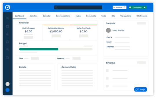
Investigation case management software provides all the data needed for the investigation. Many companies have found that using a software application is an excellent way to track cases from initiation to resolution. Because of the sensitive nature of any case, having a software tool allows you to describe your process for the investigation and then focus on making sure the initiators of any case are happy and kept safe while maintaining your reputation and keeping status.

If you’re a practicing lawyer in need of an efficient system for any investigation, be it business-related, money-laundering, fraud, or even background check of employees, do consider investigating case management software for the below-mentioned reasons.

Reasons to Use Investigation Case Management Software

Consolidates Data

Important data that can be utilized as actionable intelligence can be centrally managed from the investigation software. This spells out convenience because as the legal field involves so much data handling, and that too in different locations – some hard copy and some soft copy, such a consolidation under a powerful system makes work much easier. It also allows one-stop access to all the appropriate data. The investigation case management software can take data from various systems and information sources that were previously separated from each other under one software.

Simplification of Process

Investigation management software facilitates the process simply by ensuring more organization. Once the data is consolidated, it can be organized, making it easier to analyze and categorize the data. Data is thereby assigned as essential or not. Investigation case management software allows for the sifting of data.

Confidentiality

Investigation case management software restricts access to just users who have the access information. Thereby ensuring that sensitive data does in no way get revealed. Such an option is, for apparent reasons, important in the context of an investigation, where evidence tampering, fraud, and destruction of evidence are all genuine threats to the integrity of the investigation. In such cases, investigation software allows for better security of information gathered.

Saves Time

Investigation case management software helps in managing and accessing data. Typically, the legal field involves scattered data that needs to be pieced together and sometimes escapes any primary forms of organization and efficiency. This causes a lot of time spent, which can be saved by using investigation case management software. As we’ve mentioned above, the software allows us to collate, organize, and analyze the data required for the investigation. This, in turn, will enable us to save time.

ICAC software automates processes and has improved accuracy, real-time reporting, and universal access. This also helps in saving valuable time, which can then be diverted elsewhere.

Improved Collaboration

Investigation case management software allows for cross-department/cross-platform sharing and collaboration. It is easy to see how such software could ease the sharing of information between parties involved and law enforcement with such a tool.

Saves Money

Case management for law enforcement helps in facilitating interactions and communication. It gives an interface that allows for higher efficiency and does away with paperwork reliance. Thus, investigation case management software is a one-time investment that helps the user to save money with its features, which are unique to each software.

Conclusion

Investigation management software is one of the many types of software revolutionizing how lawyers and law enforcement agencies conduct their tasks. For reasons earlier mentioned, the tasks can now be performed with enhanced ease and efficiency. 

[synatkeam]

Assignment week 4

## load the library

import numpy as np

import pandas as pd

import seaborn import matplotlib.pyplot as plt

## read the data

import pandas import numpy radioimmuno= pandas.read_csv("radioimmuno.csv") radioimmuno

# checking the format of your variables

radioimmuno['Mouse.Identification'].dtype radioimmuno['Treatment.group'].dtype radioimmuno['Surviveal.day'].dtype radioimmuno['Number.of.T.cell'].dtype

radioimmuno['Percentage_of_T.cell.activation'].dtype

# setting variables to numeric

radioimmuno['Surviveal.day'] = pandas.to_numeric(radioimmuno['Surviveal.day']) radioimmuno['Number.of.T.cell'] = pandas.to_numeric(radioimmuno['Number.of.T.cell']) radioimmuno['Percentage_of_T.cell.activation'] = pandas.to_numeric(radioimmuno['Percentage_of_T.cell.activation'])

## Creating graph

seaborn.catplot(x='Treatment.group', y='Surviveal.day', data=radioimmuno, kind="bar", ci=None) plt.xlabel('radiation group') plt.ylabel('number of day')

## Interpretation and summary

The bargraph here demonstrated that group that received radiotherapy and immunotherapy combination survived longer than group that received just radiation alone. This suggested that adding radiotherapy improved the efficacy of immunotherapy in cancer.

[mycloudhospitality]

How to Improve Profits with Hotel Data Management?

In the hotel business, there are few things more valuable than data and at the same time, most hoteliers are not able to use the data to improve the profits at their property. Every day, every moment, a hotel business produces data. From the activities of the guests, to staff movements in cleaning the rooms, and addition of new inventory to the kitchens, every activity is data. This data can be further used by a professional management team to improve the performance of various facets of the hotel’s operations.

Without a hotel management system, there is a chance that this information will be lost and not generate any profits for the hotel. But with a reliable hotel software in place, this data can be utilized to maximize profitability and improve guest experience through the property. The data can be used to predict customer behavior, identify profit and loss making channels, add to profits and much more. With the right analytical framework and the ideal tools, hotels can derive actionable business intelligence from the data points.

Let’s dive in a little deeper to understand the kinds of data that can be utilized and how hotels can make the best use of this data.

What Are the Different Types of Data that Can Be Collected?

Booking Data

This data can include basic information about distribution channels, duration of stay, room history, abandonment rate, and more. Once you analyze the data, you will get a better understanding of how your hotel property is performing and which areas need improvement. You can find out which rooms are doing well in a particular season and price them accordingly while highlighting those rooms in your marketing efforts.

Guest Data

Important data about the guests can range from demographics, guest’s preferences about food and beverage, booking history, payment preferences, and contact information. This data can help you to personalize services for the guests to enhance their experience at the hotel. You can also use the data to offer rewards and incentives to guests so that they are more inclined to choose your property for stay during their next vacation.

Housekeeping Data

In the current time and age, hotels need to put more emphasis on ensuring that their rooms are clean and sanitized at regular intervals. This data can include the number of housekeeping staff, number of rooms cleaned, speed of cleaning, supplies used, laundry expenses and more. By using an advanced hotel software, managers can zero in on the gaps in the housekeeping schedule and adjust the team’s workflow accordingly.

Social Media Data

In the age of social media, hotels need to keep an eye on their reputation across various social media channels. Social media heatmap can help you to figure out where your guests are coming from, you can also collaborate the ratings from different OTAs on a single dashboard to find out the areas that need improvement.

How Does a Hotel Software Allow Better Data Management?

A hotel property generates data 24/7 and it is critical to collect and analyze this data for better decision making. Whether it is the front desk, guest activities, PoS software, channel manager or housekeeping staff, all activities in the hotel offer information that can be used. Luckily, hotel management software can help to bring together this data in a comprehensive manner so that managers can base their decision making on the available data. Here are some ways to manage data in a structured and balanced manner.

Data Collection from Multiple Sources - A PMS can have modules added into it so that you can gather data from various points of interest. Whether it is your OTA, booking agency, or social network, you can get data that refer to your property on a combined dashboard. You can also configure the hotel software to send emails and texts to guests once they have checked out. Guests can then fill a short survey with their feedback about their experience at the property.

Integration with Present Systems - When you are using a state-of-the-art PMS, you can get integration options for various third party tools to exchange data. The data sharing can happen when you add modules such as PoS (point of sale), RMS (Revenue Management System), CRM (Customer Relationship Management system) and more with the hotel software. What’s more, as the software operates in the cloud, you can also get modern APIs for new modules and add them to your dashboard.

Data Filtration - When data is collected from multiple sources, there are bound to be instances of data duplication or incomplete data. A quality software will be able to classify data that is useful and complete. You can further use filters and segregate the data according to the reports you need.

Data Analysis - Once the data is filtered, it needs to be analyzed. Modern hotel management software comes with business intelligence tools that offer in-depth analytics for all kinds of data. You can further customize the software to suit the needs of your business. With analysis, you can generate reports through the hotel management software and visualize the data as needed.

Conclusion

If you are not leveraging the data that is gathered in your hotel, you are simply leaving money on the table. Every hotel property can be further optimized to reduce costs and increase profits, so how are you going to do it? You can do it by using the hotel software offered by mycloud Hospitality.

With more than a decade and a half’s experience in providing IT solutions to businesses around the world, the team at mycloud Hospitality offers solutions that are tailor made to the needs of their hospitality clients. Interested in learning more? Check out https://www.mycloudhospitality.com/

.

[coursera2022]

Multiple Regression

Assignment: Test a Multiple Regression Model

Following is the Python program I wrote to fulfill the third assignment of the Regression Modeling in Practice online course.

I decided to use Jupyter Notebook as it is a pretty way to write code and present results.

Assignment research question

Using the Gapminder database, I would like to see if there is a relationship between the income per person (explanatory variable) and the residential consumption of electricity (response variable).

The following variables will be tested also to improve the prediction model and figure out potential confounders:

Employment rate (total employees age of 15+)

Oil consumption per person (tonnes per year per person)

Urban rate (Urban population in %)

Data management

For the question I'm interested in, the countries for which data are missing will be discarded. As missing data in Gapminder database are replaced directly by NaN no special data treatment is needed.

In [2]:# Magic command to insert the graph directly in the notebook%matplotlib inline # Load a useful Python libraries for handling dataimport pandas as pd import numpy as np import statsmodels.api as sm import statsmodels.formula.api as smf import scipy.stats as stats import seaborn as sns import matplotlib.pyplot as plt from IPython.display import Markdown, display

In [3]:# Read the data data_filename = r'gapminder.csv' data = pd.read_csv(data_filename, low_memory=False) data = data.set_index('country')

General information on the Gapminder data

In [4]:display(Markdown("Number of countries: {}".format(len(data))))

Number of countries: 213

Data managment

In order to carry out the regression analysis, we need to center the potential explanatory variables.

In [5]:subdata = (data[['incomeperperson', 'relectricperperson', 'employrate', 'oilperperson', 'urbanrate']] .assign(income=lambda x: pd.to_numeric(x['incomeperperson'], errors='coerce'), electricity=lambda x: pd.to_numeric(x['relectricperperson'], errors='coerce'), employ=lambda x: pd.to_numeric(x['employrate'], errors='coerce'), oil=lambda x: pd.to_numeric(x['oilperperson'], errors='coerce'), urban=lambda x: pd.to_numeric(x['urbanrate'], errors='coerce')) .dropna()) display(Markdown("Number of countries after discarding countries with missing data: {}".format(len(subdata)))) centered_data = (subdata.assign(income_c=lambda x: x['income'] - subdata['income'].mean(), employ_c=lambda x: x['employ'] - subdata['employ'].mean(), oil_c=lambda x: x['oil'] - subdata['oil'].mean(), urban_c=lambda x: x['urban'] - subdata['urban'].mean()))

Number of countries after discarding countries with missing data: 61

Let's check the variables are well centered

In [6]:display(Markdown("Mean of income per person after centering: {:3g}".format(centered_data['income_c'].mean()))) display(Markdown("Mean of employment rate after centering: {:3g}".format(centered_data['employ_c'].mean()))) display(Markdown("Mean of oil consumption per person after centering: {:3g}".format(centered_data['oil_c'].mean()))) display(Markdown("Mean of urban rate after centering: {:3g}".format(centered_data['urban_c'].mean())))

Mean of income per person after centering: -1.77426e-12

Mean of employment rate after centering: -2.56261e-15

Mean of oil consumption per person after centering: 5.49651e-16

Mean of urban rate after centering: 1.9569e-14

Bivariate distribution

Before looking at the multiple regression analysis, an polynomial regression will be applied on the data to see if it fits better the results.

In [7]:sns.regplot(x='income_c', y='electricity', data=centered_data) sns.regplot(x='income_c', y='electricity', order=2, data=centered_data) plt.xlabel('Centered income per person (2000 US$)') plt.ylabel('Residential electricity consumption (kWh)') plt.title('Scatterplot for the association between the income and the residential electricity consumption');

OLS regression model

Test the linear regression model.

In [8]:reg1 = smf.ols('electricity ~ income_c', data=centered_data).fit() reg1.summary()

Out[8]:

OLS Regression ResultsDep. Variable:electricityR-squared:0.402Model:OLSAdj. R-squared:0.392Method:Least SquaresF-statistic:39.69Date:Sun, 17 Jul 2016Prob (F-statistic):4.08e-08Time:19:02:59Log-Likelihood:-530.88No. Observations:61AIC:1066.Df Residuals:59BIC:1070.Df Model:1Covariance Type:nonrobustcoefstd errtP>|t|[95.0% Conf. Int.]Intercept1626.2603189.6708.5740.0001246.731 2005.790income_c0.09500.0156.3000.0000.065 0.125Omnibus:80.246Durbin-Watson:2.135Prob(Omnibus):0.000Jarque-Bera (JB):1091.497Skew:3.660Prob(JB):9.65e-238Kurtosis:22.387Cond. No.1.26e+04

Test a second order polynomial regression model.

In [9]:reg2 = smf.ols('electricity ~ income_c + I(income_c**2)', data=centered_data).fit() reg2.summary()

Out[9]:

OLS Regression ResultsDep. Variable:electricityR-squared:0.413Model:OLSAdj. R-squared:0.393Method:Least SquaresF-statistic:20.43Date:Sun, 17 Jul 2016Prob (F-statistic):1.92e-07Time:19:02:59Log-Likelihood:-530.31No. Observations:61AIC:1067.Df Residuals:58BIC:1073.Df Model:2Covariance Type:nonrobustcoefstd errtP>|t|[95.0% Conf. Int.]Intercept1904.3071325.7615.8460.0001252.225 2556.389income_c0.11170.0225.0950.0000.068 0.156I(income_c ** 2)-1.758e-061.68e-06-1.0490.298-5.11e-06 1.6e-06Omnibus:76.908Durbin-Watson:2.098Prob(Omnibus):0.000Jarque-Bera (JB):912.307Skew:3.504Prob(JB):7.85e-199Kurtosis:20.602Cond. No.3.92e+08

From the second OLS analysis, we can see that the coefficient corresponding to the second order term has a p-value of 0.3 > 0.05. Therefore we should keep only the linear term for our primary relation.

Multiple regression

The multiple regression will be now carried out.

In [10]:reg3 = smf.ols('electricity ~ income_c + oil_c + employ_c + urban_c', data=centered_data).fit() reg3.summary()

Out[10]:

OLS Regression ResultsDep. Variable:electricityR-squared:0.452Model:OLSAdj. R-squared:0.412Method:Least SquaresF-statistic:11.53Date:Sun, 17 Jul 2016Prob (F-statistic):6.76e-07Time:19:03:00Log-Likelihood:-528.25No. Observations:61AIC:1067.Df Residuals:56BIC:1077.Df Model:4Covariance Type:nonrobustcoefstd errtP>|t|[95.0% Conf. Int.]Intercept1626.2603186.4708.7210.0001252.716 1999.804income_c0.07580.0203.8830.0000.037 0.115oil_c123.7307135.5640.9130.365-147.837 395.298employ_c48.676525.9011.8790.065-3.209 100.562urban_c2.357113.8640.1700.866-25.415 30.129Omnibus:62.530Durbin-Watson:2.146Prob(Omnibus):0.000Jarque-Bera (JB):537.653Skew:2.704Prob(JB):1.78e-117Kurtosis:16.502Cond. No.1.26e+04

Unexpectedly all explanatory variables except the primary one (income per person) should be discarded as their coefficients have p-values higher than 0.05.

Finally we will look at the diagnostic graphs

Q-Q plot for normality

In [11]:fig = sm.qqplot(reg1.resid, line='r')

The residuals do not follow correctly the line. Especially on the second half of the data. As our model is a single linear regression between residential electricity consumption and income per person, this means that the model is a poor predicator for country having larger income.

Residuals plot

In [12]:stdres = pd.DataFrame(reg1.resid_pearson) plt.plot(stdres, 'o') plt.axhline(y=0, color='r') plt.ylabel('Standardized Residual') plt.xlabel('Observation Number');

The previous plot highlights only one clear extreme outlier. So this confirm that the model is fine and could be improve.

Partial regression plots

In [13]:fig = plt.figure(figsize=(12,8)) sm.graphics.plot_regress_exog(reg3, 'urban_c', fig);

In [19]:fig = plt.figure(figsize=(12,8)) sm.graphics.plot_regress_exog(reg3, 'oil_c', fig);

In [20]:fig = plt.figure(figsize=(12,8)) sm.graphics.plot_regress_exog(reg3, 'employ_c', fig);

The partial regression plots above are shown for the sake of the assignement as all variables but the income per person are non-significant in the multiple regression model. They all show that some extreme outliers will be present.

And the partial plot against the urban rate has a horizontal partial regression line. This confirms that urban rate cannot improve the model.

Leverage plot

In [14]:sm.graphics.influence_plot(reg1);

The leverage plot above shows that our extreme outlier United Arab Emirates does not have a strong influence on the estimation of the model coefficient. On the contrary Norway, the second border highest residual, has a important influence on the model estimation.

Analysis of trouble case

To conclude this assignment, I would to take the same question but taking the oil consumption as primary explanatory variables.

Let's first see if a second order fits better than the linear regression model.

In [15]:sns.regplot(x='oil_c', y='electricity', data=centered_data); sns.regplot(x='oil_c', y='electricity', order=2, data=centered_data) plt.xlabel('Centered oil consumption per person (tonnes)') plt.ylabel('Residential electricity consumption (kWh)') plt.title('Scatterplot for the association between the oil and the residential electricity consumption');

In [16]:reg_oil1 = smf.ols('electricity ~ oil_c', data=centered_data).fit() reg_oil1.summary()

Out[16]:

OLS Regression ResultsDep. Variable:electricityR-squared:0.199Model:OLSAdj. R-squared:0.185Method:Least SquaresF-statistic:14.64Date:Sun, 17 Jul 2016Prob (F-statistic):0.000317Time:19:03:39Log-Likelihood:-539.82No. Observations:61AIC:1084.Df Residuals:59BIC:1088.Df Model:1Covariance Type:nonrobustcoefstd errtP>|t|[95.0% Conf. Int.]Intercept1626.2603219.5837.4060.0001186.877 2065.644oil_c487.8025127.5053.8260.000232.666 742.939Omnibus:47.149Durbin-Watson:1.867Prob(Omnibus):0.000Jarque-Bera (JB):273.869Skew:1.975Prob(JB):3.39e-60Kurtosis:12.599Cond. No.1.72

In [17]:reg_oil2 = smf.ols('electricity ~ oil_c + I(oil_c**2)', data=centered_data).fit() reg_oil2.summary()

Out[17]:

OLS Regression ResultsDep. Variable:electricityR-squared:0.595Model:OLSAdj. R-squared:0.581Method:Least SquaresF-statistic:42.58Date:Sun, 17 Jul 2016Prob (F-statistic):4.18e-12Time:19:03:39Log-Likelihood:-519.02No. Observations:61AIC:1044.Df Residuals:58BIC:1050.Df Model:2Covariance Type:nonrobustcoefstd errtP>|t|[95.0% Conf. Int.]Intercept2079.9567168.62012.3350.0001742.428 2417.486oil_c1617.3225175.6839.2060.0001265.655 1968.990I(oil_c ** 2)-152.975820.316-7.5300.000-193.643 -112.309Omnibus:46.176Durbin-Watson:1.686Prob(Omnibus):0.000Jarque-Bera (JB):230.695Skew:2.004Prob(JB):8.04e-51Kurtosis:11.643Cond. No.19.1

From the OLS analysis, the second order regression fits better the results. But the outlier far on the right seems to deteriorate the accuracy of the linear regression coefficient.

This is confirm by the leverage plot below. Singapore has a strong influence on the regression model. This country is a singularity having a huge oil consumption but a reasonable residential electricity consumption.

In [18]:sm.graphics.influence_plot(reg_oil1);

Anyway the multiple regression shows that oil consumption is not a significant explanatory variable of the residential electricity consumption. Indeed in this case income per person is a cofounder; that is the real explanatory variable.

Conclusion

In this assignment we have seen that only our primary explanatory variable (income per person) is a good to build a regression model on. However the R-Squared value being 0.4, there is still 60% of the electricity consumption variations not explain with the model; in particular the model performs poorly for country with higher income.

In the latter part, we use the tools described in this week to the trouble than can be raised by outlier data.

[codehunter]

Global variable and python flask [duplicate]

This question already has answers here:

Are global variables thread-safe in Flask? How do I share data between requests? (4 answers)

Closed last year.

What i want to do is just display the firstevent from one API. The variable is called “firstevent” and the value should display on the webpage. But firstevent is inside a def, so i change it into a global variable and hope it can be used across different functions. But it shows “NameError: global name 'firstevent' is not defined”. This is what I am doing:

define a global variable

global firstevent

send this variable a random value, it supposed to be events['items'][1]['end']

firstevent = 1

displaying firstevent’s value on website.

@app.route("/")def index(): return 'User %s' % firstevent

I am not sure what’s happening now, maybe it’s a scope issue? I have check many answers online but still cannot find the solution.

Here are the details(not the whole code)

import os# Retrieve Flask, our framework# request module gives access to incoming request dataimport argparseimport httplib2import osimport sysimport jsonfrom flask import Flask, requestfrom apiclient import discoveryfrom oauth2client import filefrom oauth2client import clientfrom oauth2client import toolsfrom apiclient.discovery import buildfrom oauth2client.client import OAuth2WebServerFlowimport httplib2global firstevent app = Flask(__name__)def main(argv): # Parse the command-line flags. flags = parser.parse_args(argv[1:]) # If the credentials don't exist or are invalid run through the native client # flow. The Storage object will ensure that if successful the good # credentials will get written back to the file. storage = file.Storage('sample.dat') credentials = storage.get() if credentials is None or credentials.invalid: credentials = tools.run_flow(FLOW, storage, flags) # Create an httplib2.Http object to handle our HTTP requests and authorize it # with our good Credentials. http = httplib2.Http() http = credentials.authorize(http) # Construct the service object for the interacting with the Calendar API. calendar = discovery.build('calendar', 'v3', http=http) created_event = calendar.events().quickAdd(calendarId='XXXX@gmail.com', text='Appointment at Somewhere on June 3rd 10am-10:25am').execute() events = calendar.events().list(calendarId='XXXX@gmail.com').execute() #firstevent = events['items'][1]['end'] firstevent = 1 #print events['items'][1]['end'] # Main Page Route@app.route("/")def index(): return 'User %s' % firstevent# Second Page Route@app.route("/page2")def page2(): return """<html><body> <h2>Welcome to page 2</h2> <p>This is just amazing!</p> </body></html>"""# start the webserverif __name__ == "__main__": app.debug = True app.run()

https://codehunter.cc/a/flask/global-variable-and-python-flask-duplicate