#adjacency matrix of a graph example

[fortunatelycoldengineer]

What Does Big O(N^2) Complexity Mean?

It's critical to consider how algorithms function as the size of the input increases while analyzing them. Big O notation is a crucial statistic computer scientists use to categorize algorithms, which indicates the sequence of increase of an algorithm's execution time. O(N^2) algorithms are a significant and popular Big O class, whose execution time climbs quadratically as the amount of the input increases. For big inputs, algorithms with this time complexity are deemed inefficient because doubling the input size will result in a four-fold increase in runtime.

This article will explore what Big O(N^2) means, analyze some examples of quadratic algorithms, and discuss why this complexity can be problematic for large data sets. Understanding algorithmic complexity classes like O(N^2) allows us to characterize the scalability and efficiency of different algorithms for various use cases.

Different Big Oh Notations.

O(1) - Constant Time:

An O(1) algorithm takes the same time to complete regardless of the input size. An excellent example is to retrieve an array element using its index. Looking up a key in a hash table or dictionary is also typically O(1). These operations are very fast, even for large inputs.

O(log N) - Logarithmic Time:

Algorithms with log time complexity are very efficient. For a sorted array, binary search is a classic example of O(log N) because the search space is halved each iteration. Finding an item in a balanced search tree also takes O(log N) time. Logarithmic runtime grows slowly with N.

O(N) - Linear Time:

Linear complexity algorithms iterate through the input at least once. Simple algorithms for sorting, searching unsorted data, or accessing each element of an array take O(N) time. As data sets get larger, linear runtimes may become too slow. But linear is still much better than quadratic or exponential runtimes.

O(N log N) - Log-Linear Time:

This complexity results in inefficient sorting algorithms like merge sort and heap sort. The algorithms split data into smaller chunks, sort each chunk (O(N)) and then merge the results (O(log N)). Well-designed algorithms aimed at efficiency often have log-linear runtime.

O(N^2) - Quadratic Time:

Quadratic algorithms involve nested iterations over data. Simple sorting methods like bubble and insertion sort are O(N^2). Matrix operations like multiplication are also frequently O(N^2). Quadratic growth becomes infeasible for large inputs. More complex algorithms are needed for big data.

O(2^N) - Exponential Time:

Exponential runtimes are not good in algorithms. Adding just one element to the input doubles the processing time. Recursive calculations of Fibonacci numbers are a classic exponential time example. Exponential growth makes these algorithms impractical even for modestly large inputs.

What is Big O(N^2)?

An O(N2) algorithm's runtime grows proportionally to the square of the input size N.

Doubling the input size quadruples the runtime. If it takes 1 second to run on 10 elements, it will take about 4 seconds on 20 elements, 16 seconds on 40 elements, etc.

O(N^2) algorithms involve nested iterations through data. For example, checking every possible pair of elements or operating on a 2D matrix.

Simple sorting algorithms like bubble sort, insertion sort, and selection sort are typically O(N^2). Comparing and swapping adjacent elements leads to nested loops.

Brute force search algorithms are often O(N^2). Checking every subarray or substring for a condition requires nested loops.

Basic matrix operations like multiplication of NxN matrices are O(N^2). Each entry of the product matrix depends on a row and column of the input matrices.

Graph algorithms like Floyd-Warshall for finding the shortest paths between all vertex pairs is O(N^2). Every possible path between vertices is checked.

O(N^2) is fine for small inputs but becomes very slow for large data sets. Algorithms with quadratic complexity cannot scale well.

For large inputs, more efficient algorithms like merge sort O(N log N) and matrix multiplication O(N^2.807) should be preferred over O(N^2) algorithms.

However, O(N^2) may be reasonable for small local data sets where inputs don't grow indefinitely.

If you want more learning on this topic, please read more about the complexity on our website.

[codingprolab]

EECS 560 Lab 6 undirected graph

Due to the symmetry in an undirected graph, it is only necessary to store the edge weights in the upper triangle of the adjacency matrix (above the diagonal).   For example, if you want to find the weight of the edge (5, 3), due to symmetry you can get this information by looking at the weight of (3, 5). For this lab you will randomly generate connected graphs and store their information in a one…

[kitwallace]

Non-Eulerian paths

I've been doing a bit of work on Non-Eulerian paths.  I haven't made any algorithmic progress with the non-spiraling approach Piotr Waśniowski uses for such paths, but I'm keen to continue the development of the approach using spiral paths since I believe that this yields strong structures. 

I'm using the Hierholzer algorithm to find paths in a Eulerian graph  and I've been looking at the changes needed for non-Eulerian graphs, i.e. those where the order of some vertices is odd. For graphs with only 2 odd nodes, a solution is to use pairs of layers which alternate starting nodes. In the general case  (Chinese Postman Problem)  duplicate edges are added to convert the graph to Eulerian and then Hierholzer used to solve the  resultant graph.  I hadn't actually tried this before but I've now used this approach on some simple cases. 

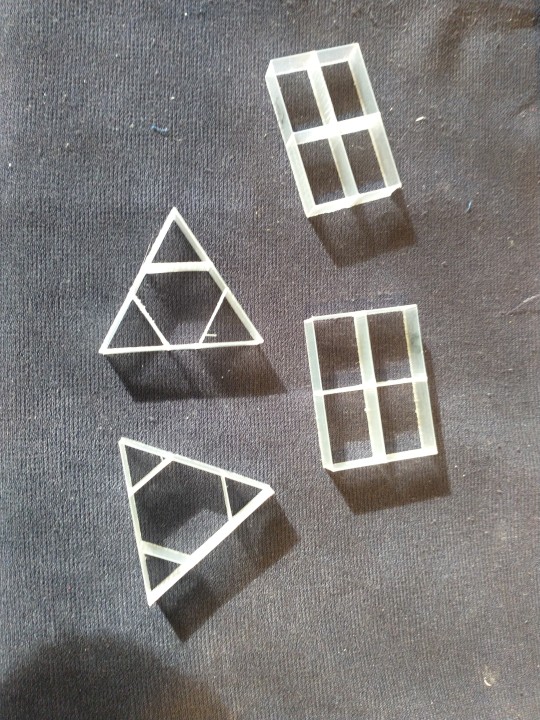
(the paths here were constructed via Turtle graphics just to test the printing - in transparent PLA)  

The hard part is to evaluate the alternative ways in which the duplicate edges can be added.  We can minimise the weighted sum of edges but for the rectangle this still leaves several choices and I need to think about how they can be evaluated.  I think immediate retracing of an edge should be avoided so perhaps maximising the distance between an edge and its reverse would be useful.

The duplicate edges cause a slight thickening and a loss of surface quality (so better if they are interior)  but I think that's a small cost to retain the spiral path. Path length for the rectangle is 25% higher  I haven't tried them with clay yet.

Modifying Hierholzer

I had originally thought that to formulate such graphs for solution by Hierholzer, each pair of duplicate edges would require an intermediate node to be added to one of the edges to create two new edges. This would be the case if the graph was stored as an NxN matrix, but my algorithm uses a list of adjacent nodes, since this allows weights and other properties to be included. Removing a node from the matrix is much faster (just changing the entry to -1) than removing the node from a list but for my typical applications efficiency is not a big issue. The list implementation requires only a simple modification to remove only the first of identical nodes. This allows duplicate edges to be used with no additional intermediate nodes.

This is test interface for the Hierholzer algorithm which accepts a list of edges.

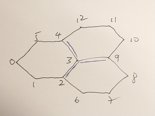
Here is an example with three hexagons:

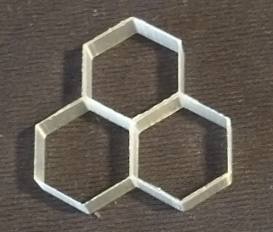
with graph

and edge list:

[ [0,1],[1,2],[2,3],[3,4],[4,5],[5,0], [3,2],[2,6],[6,7],[7,8],[8,9],[9,3], [3,9],[9,10],[10,11],[11,12],[12,4],[4,3] ]

Nodes 2,3,4 and 9 are odd. There is only one way to convert to Eulerian. We need to duplicate three edges : [3,4], [3,9],[3,2] so that nodes 4,9, and 2 become order 4 and node 3 becomes order 6. The path used to generate the printed version above was constructed as a Turtle path with only 60 degree turns:

[3, 9, 10, 11, 12, 4, 3, 2, 6, 7, 8. 9, 3, 4, 5, 0, 1, 2]

Hierholzer constructs the following path starting at the same node

[3, 2, 1, 0, 5, 4, 3, 2, 6, 7, 8, 9, 3, 9, 10, 11, 12, 4]

There is a sub-sequence [9,3,9] which indicates an immediate reversal of the path. This creates the possibility of a poor junction at node 3 and is to be avoided.

Furthermore, this path is the same regardless of the starting point. The choice of which edge amongst the available edges from a node at each step is deterministic in this algorithm but it could be non-deterministic. With this addition, after a few attempts we get :

[0, 1, 2, 3, 9, 10, 11, 12, 4, 3, 2, 6, 7, 8, 9, 3, 4, 5]

with no immediately repeated edges

This provides a useful strategy for a generate-test search: repeatedly generate a random path and evaluate the path for desirable properties , or generate N paths and choose the best.

However, this approach may not be very suitable for graphs where all nodes are odd, such as this (one of many ) from Piotr:

The edge list for this shape is

[0,1],[1,2],[2,0], [0,3],[1,4],[2,5], [3,6],[6,4],[4,7],[7,5],[5,8],[8,3], [9,10],[10,11],[11,9], [6,9],[7,10],[8,11],

duplicate the spokes

[0,3],[1,4],[2,5], [6,9],[7,10],[8,11]

Here every node is odd. The 6 spokes are duplicated. Sadly no path without a reversed edge can be found.

The simpler form with only two triangles and 3 duplicated spokes:

[ [0,1],[1,2],[2,0], [0,3],[1,4],[2,5], [0,3],[1,4],[2,5], [3,4],[4,5],[5,3] ]

does however have a solution with no reversed edges although it takes quite a few trials to find it:

[0,2,5,4,1,2,5,3,0,1,4,3]

Triangles

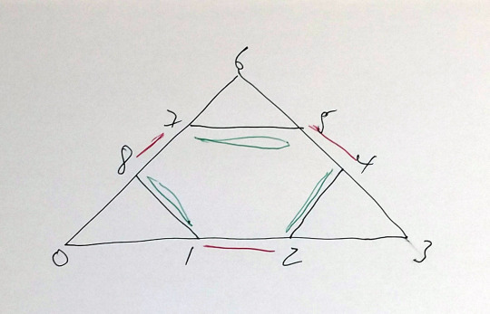
Edges can be duplicated in two ways

[[0,1],[1,2],[2,3],[3,4],[4,5],[5,6],[6,7],[7,8],[8,0] ,[2,4],[5,7],[8,1]

a) duplicating the interior edges min 4

[2,4],[5,7],[8,1]

b) duplicating the exterior edges min 6 [1,2],[4,5],[7,8]

Rectangle

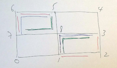
Edges can be duplicated in three different ways

[0,1],[1,2],[2,3],[3,4],[4,5],[5,6],[6,7],[7,0], [1,8],[3,8],[5,8],[7,8],

a) [1,2],[2,3], [5,6],[6,7] min 6 b) [1,8],[8,3], [5,6],[6,7] min 4 c) [1,8],[8,3], [5,8],[8,7] min 4

Automating edge duplication

The principal is straightforward: chose an odd node, find its nearest neighbour and duplicate the connecting edge(s) ;repeat until all odd nodes connected. To test various configurations, allow the choice of node and its nearest neighbour, if several, to be randomised and compute a selection evaluation from the result.

Currently the choice is based on the length of the path from each node to the revisit of that node. Path length of 2 means an immediate return and these should be avoided if possible.

Testing with clay

Whilst tests with PLA show no significant changes in appearance whilst retaining the benefits of a spiral print path, this approach has yet to be tested with clay

Postscript

A side-benefit of this work has been that I've finally fixed an edge case in my Hierholzer algorithm which has been bugging me for some years

[essaycode1]

Essay Help Made Easy

[lazar-codes]

16/06/2023 || Day 38

Random Rambles

Writing here a bit early today, but that's because I was semi-successful today! Re-implemented insertion sort and selection sort (one day I'll get them on my first try without needing to look things up), and re-implemented a graph with an adjacency matrix. Covered Breadth-First Search traversal with graphs, and went over Depth-First Search traversal. But most importantly, I decided to tackle different LeetCode questions than the one I'm currently working on. I'm currently attempting to go through the top 150 questions for interviews (titled "Top Interview 150") and was working on the "Jump Game" question for it last night, but I decided I wanted a boost in confidence so I picked a random easy and medium question about arrays and solved them! I'll get back to the "Jump Game" one later...

In other random news/thoughts, I finished university about 2 months ago and idk what it is, but I feel like I have so much energy and desire to learn new things/follow my hobbies? I'm currently going over CS concepts so that I can get a job, so I'm sure my enthusiasm to learn stuff will disappear once I do get a job, but in the meantime...I want to learn so much and do so much, but even with no job it feels like there's no time! For example, I spend most of my day covering CS topics (theory), then try to solve a LeetCode question, and by then it's 5pm. So from then on it's either work on a Frontend Mentor project or continue with The Odin Project or learn something new with regards to CS. But there's other things I want to do, like maybe play some games or watch tv or read or do art (and finally learn Blender and get better at using Procreate), but by the time programming is done it's like 9:30pm. And the easy solution is to cut down on programming, but I'm having fun doing it and I don't want to cut down! Anyways, that's me just rambling/being excited about how I finally have the drive/desire to do my hobbies/improve on them. It's really exciting, but a little annoying knowing I can't do everything at once.

[trustswitch]

Matlab tutorial

MATLAB TUTORIAL PROFESSIONAL

If X is a vector, then diff(X) returns a vector, one element shorter than X, of differences between adjacent elements:y=.y=diff(X) calculates differences between adjacent elements of X.The Syntax is: Y = diff(X) or Y = diff(X,n), n is the dimension of the derivative (such as a second derivative, third derivative, etc.) If n=1, it is the same as y=diff(x).Matlab is able to do differences and approximate derivatives, the basic function is diff.So, if you want a mathematical formula of a derivative, use a calculator or another program.Matlab can simulate both Integration and Derivative, not formulaically but by numerical approximation.The difference is: plot will plot a continuous graph stem is for the discrete graph.The most common functions for graphing are plot, stem, polar, subplot, mesh, meshc, surf, surfc, and hold on. After setting and operating on arrays, the best way to see the behavior of x and y, or x,y, and z is to graph them. You don't need to set a for loop like in other programming languages to calculate the value of each element in b.Or, you can also use b=sqrt(a), the result is same.To make an operation work on an array, just add a dot before the normal operator. After setting the variables, you can do normal operations between arrays.For example, if you want to simulate a step function: x=, then x will be: 0 0 0 0 0 1 1 1 1 1 With these two useful arrays, you can save time on setting values.The format is : zeros/ones("number of dimension", length of array) Each is an array filled with either zeros or ones. Matlab has 2 useful default arrays: zeros, and ones.Of course, you can also set each element by hand, using a space to separate each element in the row, and a semicolon to separate each row.If you want to change the step length, the format is: x=a:"length of step":b.Array Format (one dimensional): x=, a is the beginning value, b is the ending value, the default step is 1.You can use either vector or array form to store variables. One dimension arrays and vectors are almost the same in Matlab.

MATLAB TUTORIAL PROFESSIONAL

Many classes in our ECEn Department requires professional skill using matlab, such as ECEn 360, ECEn 370, ECEn 380, ECEn 483. Created by The MathWorks, MATLAB allows easy matrix manipulation, plotting of functions and data, implementation of algorithms, creation of user interfaces, and interfacing with programs in other languages. MATLAB is a numerical computing environment and programming language. This tutorial is for those who have never touched matlab before or need some review for matlab. Writer: Zixu Zhu || Email: topics below are the most important topics selected from the result of students' survey.

[coolravish]

Understanding vector, map and their uncommon implementation:Explanation with their Code

Hey guys,this is my first article on tumblr so suggestions are most welcomed, I thought of writing an article which contains precise explanation with precise code as i am not going to waste my time by speaking on why this is needed and all,So i begin my series of articles based on the responses i will be writing articles further on ds algo etc…Mainly i will try to cover implementation portion of it by using real problems as most of the sites lacks that information.In this article i am going to discuss on following topics:

Vector

Map

So lets explore and understand about them in simple words and in detail:

Vector:-Vector is basically a dynamic array.Now you might be wondering that what exactly we mean here by dynamic?

In a nutshell:-Dynamic means flexible,means size is not fixed.Like an array has constant/fixed size,so you may have question in your mind then what is the need of using vector.See it is useful in questions where we don’t have any idea about size and in array we cannot erase values at arbitrary position,whereas we can erase values in vector using vector erase function.

Now in programming it is believed that understanding the implementation part will help you in better way rather than wasting time on reading theory,

Implementation:

Vector Representation:-vector<int>v;vector<int>v(n),vector<int>v[n];

Now you saw that i wrote three representations,so what are the differences between them.

vector<int>v:-This represents that size of vector is not fixed here,it can change according to the situation. For eg-Initially size of vector is 0,and now if i did operation v.push_back(1),here push_back is used to insert value inside vector,so now size of vector will be 1,and similarly again i perform v.push_back(8),now size of vector is 8,and lets traverse the vector…so we will write for(i=0;i<v.size();i++){v[i]……}so now we can use it as an array…push_back inserts value at the end,like in above example v[0]=1,v[1]=8…Now i told you that we can erase values in vector..So if we want to erase value at desired position then apply v.erase(v.begin()+desired position).There are other ways of erasing also.

vector<int>v(n):-This is exactly same as int a[n].

vector<int>v[n]:-This means vector of vector,this one will better understand by example.

v[0].push_back(1);v[0].push_back(8);v[4].push_back(-1);

v[6].push_back(5);

So above we saw that v[0] is one vector and inside that one another vector is present of size 2 and its elements are 1 and 8 respectively.so if we want to traverse each element individually:-

for(i=0;i<v.size();i++)

{for(j=0;j<v[i].size();j++)

{

v[i][j]……//means whatever operation you want to perform can do…as v[i][j] is individual element like v[0][1]=8,its like 2d matrix.

}

}So above v.size()==3,as one is v[0],v[4],v[6],in nutshell we understand that inside one vector one other vector is present ,this is mainly used in graphs as when you will read about depth first search there you will get to know about adjacency list.

2)Map:-Very Powerful STL tool.

Lets understand map by example.Q)Say in a class we have marks of 10 students in maths exam-10,50,50,30,24,50,20,30,10,50…our question is that count no.of students corresponding to marks obtained?Means how many have scored 50,how many have scored 10 likewise……..

So if our question would have asked calculate frequency for 50 marks only then we could have solved it easily by running a loop and taking count of 50 marks students….but here we have to calculate frequency for each individual marks….so in cases like this our Map is helpful….

Implementation:

map<int,int>m1; This is representation of map.

for(i=0;i<n;i++){

m1[a[i]]++;

}

As you can see above m1[a[i]]++,so basically map is also an array which stores value in the form of key value pair…..here key is marks and value is count of students corresponding to that marks…like m1[50]=4,m1[24]=1 in above example likewise…..so you can see map is also an array but here index is not like array one,here we have one index as 24 ,one as 50 etc…and map stores index in sorted order so like when you will traverse map..then first of all m1[10] will come then m1[24] likewise…..

Now question comes how we will traverse the map?As for traversing the array,vector we have 0-index and in ordered form…so we simply run loop for(i=0;i<n;i++) and we can easily travel them ,but in the case of map as we saw that index was like 24,50,10,30 etc..and we don’t know them beforehand so how we will tackle them…..

For traversing map,set etc we use concept of iterator

What is iterator:In simple words we can say that it is a kind of pointer.Lets move on its implementation,Like here we will traverse map using iterator,its same as traversing array using simple for loop

Implementation:

map<int,int>::iterator it=m1.begin();

for(it=m1.begin();it!=m1.end();it++)

{

int k= it->first; //means it->first refers to map key which is 24,30,50 etc..

int r= it->second; //means it->second refers to map value that is m1[50] value,m1[24] value….say m1[50]=4…so it->first=50 and it->second =4..

cout<<No.of students k marks is r<<endl;

}

3. So we saw how to traverse map using iterator…and say if we want to find maximum number of students corresponding to one particular marks,then we will apply ….if(it->second>p){p=it->second;}….inside iterator loop we will use this condition….likewise anything we can do…And we will see more applications of map,set at the end after understanding pairs ,set etc……

Above one is known as ordered map as it stores unique keys…and all keys are in sorted manner….key refers to index in basic terms….Then we have unordered map which doesn’t store keys in sorted manner and then we have multimap which allows duplicating of keys,these two we will understand further in other articles..First we should be clear with basic implementation of map..Lets discuss one more final example to have better hold on implementation part of map…say we have string=”abaaabccaababa”

And our question of is maximum frequency of occurence of any substring of size 3.I hope you have idea about string and substring and if not then let me tell you in short…A substring of size 3 in above example can be-aba,aaa,baa,aab,bcc,cca,caa etc…means continuous characters of size 3 starting from any postion is substring …in simple words

Now lets move on implementation of this question….

map<string,int>m1; Here you might be wondering that why i wrote string as key,because we are going to take count of substring so key will be string and value is count so we wrote int as value…these things you need to keep in mind while implementing map.

for(i=0;i<n-2;i++)//n=s.size(),n-2 i guess you are clear as substring of size 3 so we need to take valid input or else error will be thrown…

{

m1[s.substr(i,3)]++;

}

So here in map we will have our map like m1[“aba”],m1[“caa”],m1[“baa”] likewise…..For maximum..lets traverse the loop

map<string,int>::iterator it=m1.begin();int p=0;

for(it=m1.begin();it!=m1.end();it++)

{

if(it->second>p)

{ p=it->second;

}

}

So answer of p will be 3 as m1[“aba”]=3…and one more thing if we are required to print substring then inside that if condition just add

string s1=it->first;

So we saw the basic implementation of map,then there is one more information map contains if we will write m1.size() it returns no. of unique keys our data contains,then we have this option also m1.erase(key),means if we write m1.erase(“aba”) then our m1[“aba”] …will be erased….and we can use one more function m1.find(“aba”)…lets see its implementation

map<string,int>::iterator it1 = m1.find(“aba”);

if(it1==m1.end())

{

//means key is not present }

else if(it1!=m1.end())

{

//means key is present

}

So using this m1.find() function we can check whether key is present or not,rest function you can study from this link…Like there is one function m1.upper_bound,lower_bound this all you can study from this link…

One thing i forgot to tell you that iterator can be written in other way also like

for(auto it:m1){}||for(auto it=m1.begin();it!=m1.end();it++)

Now you know we can travel map in reverse way also like as we know that we can travel array/vector in reverse manner using for(i=n-1;i≥0;i- -) similarly here we use for(auto it=m1.rbegin();it!=m1.rend();it- -)………

Then we can store map keys in descending order by using this function

map<int,int,greater<int>()>m1; Likewise there are many more operations which you will get to know while practicing.In my further articles i will try to cover some advanced implementation of maps by solving standardized questions,as i believe that by real problems we get better feel of any topic right?

3)Some Basic Thing but sometimes tricky

To understand this lets study about pairs first…

Pairs is also a kind of array where in value portion we can store two values…

Like say rishav has got 20 marks in maths and 30 marks in science,similarly rohit has got 15 marks in maths and 0 marks in science…so how we will store theses values

Implementation

pair<int,int>p1;

p1[0].first=20,p1[0].second=30;p1[1].first=15,p1[1].second=0;if 0-index is of rishav and 1-index is of rohit.

pairs we can use in many ways now lets look on deeper implementation of it….

vector<pair<pair<int,int>,int>>v;

So what this above representation implies….This means if we write

v.push_back({{20,30},40});({}is used for make_pair operation)

so v[0].first.first=20;

v[0].first.second=30;

v[1].second=40;

Likewise if we write

vector<pair<pair<int,int>,pair<int,int>>>v;

v.push_back({{20,0},{10,30}});

so in this way we can store value for above representation

which means v[0].first.first=20;

v[0].first.second=0;

v[1].second.first=10;

v[1].second.second=30;

so i guess you are getting some feeling by observing few examples above.

We can use pairs in map also like see.

map<pair<string,string>,int>m1;

m1.insert({{rohit,rishav},4});

m1[{rohit,rishav}]=4;

here key is {rohit,rishav} and value is 4.

map<int,vector<int>>m1;

what does this mean…

m1[1].push_back(4);

m1[1].push_back(-1);

m1[3].push_back(6);

m1[3].push_back(4);

so how we will traverse map in such case…

map<int,vector<int>>::iterator it=m1.begin();

for(it=m1.begin();it!=m1.end();it++)

{

for(j=0;j<it->second.size();j++)

{

if(it->second[j] ) //so this it->second[j] this term tells us the values present inside the vector like m1[1] contains -1,4 etc…..likewise…so in this way we can traverse the map…for this case

}

}

We can have many operations like this say

map<pair<int,int>,vector<int>>m1;

map<int,set<int>>m1;

map<int,multiset<int>>m1;

map<string,pair<string,int>>m1;

etc…..

Set/multiset we will discuss in further articles….

Suggestions are welcomed

[codezclub]

C Program to find Path Matrix by powers of Adjacency matrix

Path Matrix by powers of Adjacency Matrix Write a C Program to find Path Matrix by powers of Adjacency Matrix. Here’s simple Program to find Path Matrix by powers of Adjacency Matrix in C Programming Language. Adjacency Matrix:  Adjacency Matrix is a 2D array of size V x V where V is the number of vertices in a graph. Let the 2D array be adj[][], a slot adj[i][j] = 1 indicates that there is an…

[creativecoding]

Graphs and decision trees in Python

A pair of nodes are connected by a single path.

Decision trees are great for finding solutions. The trunk is at the top and the the branches at the bottom - very Australian.

But, how are decision trees useful?

(Computer) networks require algorithms to move information around.

Financial networks - moving around money

Sewage networks - moving water around

Decision trees can determine which path to take when executing the algorithm that moves information.

Graphs

Graphs can capture interesting relationships with this data.

The min flow or max cut problem identifies which clusters in a graph have a lot of interaction between each-other but not with many (or any) other clusters.

Inference option. Is there a sequence of edges to get from A to B. Can I find the least expensive (meaning shortest) path?

The graph partition problem. Not all nodes have connections with every other node.

This is finding and isolating different sets of connections.

Min cut max flow - an efficient way of separating highly connected elements, the things that connect a lot in a sub-graph.

Graphs (graph theories) are used by us everyday in the forms of travel maps such as on the tube etc.

Di graph (directed graph) the edges pass in one direction - almost obvious, I know.

Nodes or vertices become points of intersections, places to make a choice or has terminals.

Edges would be connections between points - the roads on which we could drive. Each edge would have a weight.

Choices that remain:

What’s the expected time between a source and a destination?

What’s the distance between the two?

What’s the average speed of travel?

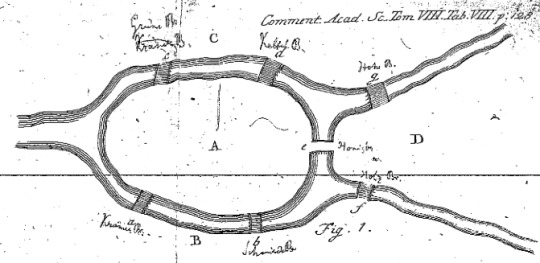
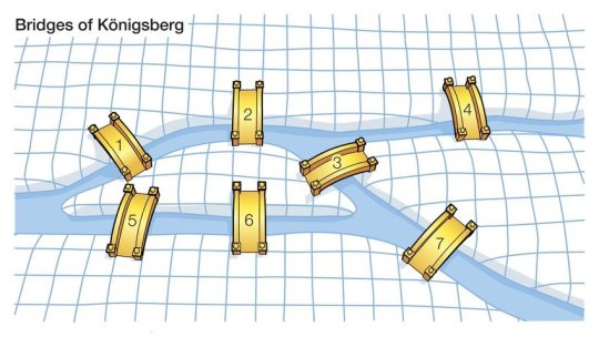
Thinking about navigation in graph systems incorporated within history from 1700′s. The image above is from ‘Solutio problematis ad geometriam situs pertinentis,’ Eneström 53 [source: MAA Euler Archive]

Bridges of Königsberg which has seven bridges that connect it’s rivers and islands - is it possible to take a walk that traverses each of the seven bridges exactly ONCE.

Leonhard Euler, a great Swiss mathematician said, “make each island a node, each bridge is an undirected edge”.

This eliminates irrelevant details about the size and focuses on the connections present, testing the point of crossing only once.

Euler's Proof and Graph Theory

When reading Euler’s original proof, one discovers a relatively simple and easily understandable work of mathematics; however, it is not the actual proof but the intermediate steps that make this problem famous.  Euler’s great innovation was in viewing the Königsberg bridge problem abstractly, by using lines and letters to represent the larger situation of landmasses and bridges.  He used capital letters to represent landmasses, and lowercase letters to represent bridges.

This was a completely new type of thinking for the time, and in his paper, Euler accidentally sparked a new branch of mathematics called graph theory, where a graph is simply a collection of vertices and edges.

Today a path in a graph, which contains each edge of the graph once and only once, is called an Eulerian path, because of this problem. From the time Euler solved this problem to today, graph theory has become an important branch of mathematics, which guides the basis of our thinking about networks.

An easy graph would be: latitude and longitude

We want to extract things away from the graph so let’s represent the nodes as objects - using classes for these.

For now, the only information to store a name (which is currently just a string) inherits from the base Python object class.

Init function used to create instances of nodes.

Store inside each instance - in other words inside of self - under the variable name of whatever was passed in as the name of that node.

If we have ways to create things with a name we need ways to get them back out. So we can select it back out by asking an instance of a node “what is your name?” by calling getName, it will return that value.

Within the class edge we’d see:

class           Edge(object):

              def _init_(self, src, dest):

                    “““Assumes src and dest are nodes”““

                    self.src = src

                    self.dest = dest

             def getSource(self) :

                    return self.src

             def getDestination(self) :

                   return self.dest

            def _str_(self):

                  return self.src.getName() + ‘->’\

                            + self.dest.getName()

To print things out we’re just gonna print name. This allows us to create as many nodes as we like.

Edges connect up two nodes - allowing us to create a fairly straightforward construction of a class. Again, it’s going to inherit from the base Python object. To create an instance of an edge we will assume in the example above that the arguments passed in (source and destination) are nodes.

This is shown after the init function.

Not names, nodes - the actual instances of the object class. So inside of the edge, we set internal variables for each instance of the edge source and destination. The get source and destination allows us to get those variables back out. The last part asks to print the name of the source then an arrow and then the destination.

So here, given an instance of an edge, we can print it and it will retrieve the source or the node associated with the source inside the instance. The opened and closed parens () is used to call it.

From this we can decide how to represent the graph, starting with a di-graph which has edges that pass in once direction. Given all the sources and all the destinations we can just create an adjacency matrix.

[highgradewriters22]

What in your opinion is the single most important motivation for the development of hashing schemes while there already are other techniques that can be used to realize the same functionality provided by hashing  methods? 

Given a directed graph, described with the set of vertices and the set of edges,  · Draw the picture of the graph· Give an example of a path, a simple path, a cycle· Determine whether the graph is connected or disconnected· Give the matrix representation of the graph· Give the adjacency lists representation of the graphEssay Question: What in your opinion is the single most important motivation…

[viswatechynology]

DFS

Depth-First Search Algorithm

The depth-first search or DFS algorithm traverses or explores data structures, such as trees and graphs. The algorithm starts at the root node (in the case of a graph, you can use any random node as the root node) and examines each branch as far as possible before backtracking.

When a dead-end occurs in any iteration, the Depth First Search (DFS) method traverses a network in a deathward motion and uses a stack data structure to remember to acquire the next vertex to start a search.

Following the definition of the dfs algorithm, you will look at an example of a depth-first search method for a better understanding.

Example of Depth-First Search Algorithm

The outcome of a DFS traversal of a graph is a spanning tree. A spanning tree is a graph that is devoid of loops. To implement DFS traversal, you need to utilize a stack data structure with a maximum size equal to the total number of vertices in the graph.

To implement DFS traversal, you need to take the following stages.

Step 1: Create a stack with the total number of vertices in the graph as the size.

Step 2: Choose any vertex as the traversal’s beginning point. Push a visit to that vertex and add it to the stack.

Step 3 — Push any non-visited adjacent vertices of a vertex at the top of the stack to the top of the stack.

Step 4 — Repeat steps 3 and 4 until there are no more vertices to visit from the vertex at the top of the stack.

Read More

Step 5 — If there are no new vertices to visit, go back and pop one from the stack using backtracking.

Step 6 — Continue using steps 3, 4, and 5 until the stack is empty.

Step 7 — When the stack is entirely unoccupied, create the final spanning tree by deleting the graph’s unused edges.

Consider the following graph as an example of how to use the dfs algorithm.

Step 1: Mark vertex A as a visited source node by selecting it as a source node.

· You should push vertex A to the top of the stack.

Step 2: Any nearby unvisited vertex of vertex A, say B, should be visited.

· You should push vertex B to the top of the stack.

Step 3: From vertex C and D, visit any adjacent unvisited vertices of vertex B. Imagine you have chosen vertex C, and you want to make C a visited vertex.

· Vertex C is pushed to the top of the stack.

Step 4: You can visit any nearby unvisited vertices of vertex C, you need to select vertex D and designate it as a visited vertex.

· Vertex D is pushed to the top of the stack.

Step 5: Vertex E is the lone unvisited adjacent vertex of vertex D, thus marking it as visited.

· Vertex E should be pushed to the top of the stack.

Step 6: Vertex E’s nearby vertices, namely vertex C and D have been visited, pop vertex E from the stack.

Read More

Step 7: Now that all of vertex D’s nearby vertices, namely vertex B and C, have been visited, pop vertex D from the stack.

Step 8: Similarly, vertex C’s adjacent vertices have already been visited; therefore, pop it from the stack.

Step 9: There is no more unvisited adjacent vertex of b, thus pop it from the stack.

Step 10: All of the nearby vertices of Vertex A, B, and C, have already been visited, so pop vertex A from the stack as well.

Now, examine the pseudocode for the depth-first search algorithm in this.

Pseudocode of Depth-First Search Algorithm

Pseudocode of recursive depth-First search algorithm.

Depth_First_Search(matrix[ ][ ] ,source_node, visited, value)

{

If ( sourcce_node == value)

return true // we found the value

visited[source_node] = True

for node in matrix[source_node]:

If visited [ node ] == false

Depth_first_search ( matrix, node, visited)

end if

end for

return false //If it gets to this point, it means that all nodes have been explored.

//And we haven’t located the value yet.

}

Pseudocode of iterative depth-first search algorithm

Depth_first_Search( G, a, value): // G is graph, s is source node)

stack1 = new Stack( )

stack1.push( a ) //source node a pushed to stack

Mark a as visited

while(stack 1 is not empty): //Remove a node from the stack and begin visiting its children.

B = stack.pop( )

If ( b == value)

Return true // we found the value

Push all the uninvited adjacent nodes of node b to the Stack

Read More

For all adjacent node c of node b in graph G; //unvisited adjacent

If c is not visited :

stack.push(c)

Mark c as visited

Return false // If it gets to this point, it means that all nodes have been explored.

//And we haven’t located the value yet.

Complexity Of Depth-First Search Algorithm

The time complexity of depth-first search algorithm

If the entire graph is traversed, the temporal complexity of DFS is O(V), where V is the number of vertices.

· If the graph data structure is represented as an adjacency list, the following rules apply:

· Each vertex keeps track of all of its neighboring edges. Let’s pretend there are V vertices and E edges in the graph.

· You find all of a node’s neighbors by traversing its adjacency list only once in linear time.

· The sum of the sizes of the adjacency lists of all vertices in a directed graph is E. In this example, the temporal complexity is O(V) + O(E) = O(V + E).

· Each edge in an undirected graph appears twice. Once at either end of the edge’s adjacency list. This case’s temporal complexity will be O(V) + O (2E) O(V + E).

· If the graph is represented as adjacency matrix V x V array:

· To find all of a vertex’s outgoing edges, you will have to traverse a whole row of length V in the matrix.

Read More

· Each row in an adjacency matrix corresponds to a node in the graph; each row stores information about the edges that emerge from that vertex. As a result, DFS’s temporal complexity in this scenario is O(V * V) = O. (V2).

The space complexity of depth-first search algorithm

Because you are keeping track of the last visited vertex in a stack, the stack could grow to the size of the graph’s vertices in the worst-case scenario. As a result, the complexity of space is O. (V).

After going through the complexity of the dfs algorithm, you will now look at some of its applications.

Application Of Depth-First Search Algorithm

The minor spanning tree is produced by the DFS traversal of an unweighted graph.

1. Detecting a graph’s cycle: A graph has a cycle if and only if a back edge is visible during DFS. As a result, you may run DFS on the graph to look for rear edges.

2. Topological Sorting: Topological Sorting is mainly used to schedule jobs based on the dependencies between them. In computer science, sorting arises in instruction scheduling, ordering formula cell evaluation when recomputing formula values in spreadsheets, logic synthesis, determining the order of compilation tasks to perform in makefiles, data serialization, and resolving symbols dependencies linkers.

3. To determine if a graph is bipartite: You can use either BFS or DFS to color a new vertex opposite its parents when you first discover it. And check that each other edge does not connect two vertices of the same color. A connected component’s first vertex can be either red or black.

4. Finding Strongly Connected Components in a Graph: A directed graph is strongly connected if each vertex in the graph has a path to every other vertex.

5. Solving mazes and other puzzles with only one solution:By only including nodes the current path in the visited set, DFS is used to locate all keys to a maze.

6. Path Finding: The DFS algorithm can be customized to discover a path between two specified vertices, a and b.

· Use s as the start vertex in DFS(G, s).

· Keep track of the path between the start vertex and the current vertex using a stack S.

Read More

· Return the path as the contents of the stack as soon as destination vertex c is encountered.

Finally, in this tutorial, you will look at the code implementation of the depth-first search algorithm.

Code Implementation Of Depth-First Search Algorithm

#include <stdio.h>

#include <stdlib.h>

#include <stdlib.h>

int source_node,Vertex,Edge,time,visited[10],Graph[10][10];

void DepthFirstSearch(int i)

{

int j;

visited[i]=1;

printf(“ %d->”,i+1);

for(j=0;j<Vertex;j++)

{

if(Graph[i][j]==1&&visited[j]==0)

DepthFirstSearch(j);

}

}

int main()

{

int i,j,v1,v2;

printf(“\t\t\tDepth_First_Search\n”);

printf(“Enter the number of edges:”);

scanf(“%d”,&Edge);

printf(“Enter the number of vertices:”);

scanf(“%d”,&Vertex);

for(i=0;i<Vertex;i++)

{

for(j=0;j<Vertex;j++)

Graph[i][j]=0;

}

for(i=0;i<Edge;i++)

{

printf(“Enter the edges (V1 V2) : “);

scanf(“%d%d”,&v1,&v2);

Graph[v1–1][v2–1]=1;

}

for(i=0;i<Vertex;i++)

{

for(j=0;j<Vertex;j++)

printf(“ %d “,Graph[i][j]);

printf(“\n”);

}

printf(“Enter the source: “);

scanf(“%d”,&source_node);

DepthFirstSearch(source_node-1);

return 0;

}

[viswatech]

DFS Algorithm

 Depth-First Search Algorithm 

The depth-first search or DFS algorithm traverses or explores data structures, such as trees and graphs. The algorithm starts at the root node (in the case of a graph, you can use any random node as the root node) and examines each branch as far as possible before backtracking.

When a dead-end occurs in any iteration, the Depth First Search (DFS) method traverses a network in a deathward motion and uses a stack data structure to remember to acquire the next vertex to start a search.

Following the definition of the dfs algorithm, you will look at an example of a depth-first search method for a better understanding.

Example of Depth-First Search Algorithm 

The outcome of a DFS traversal of a graph is a spanning tree. A spanning tree is a graph that is devoid of loops. To implement DFS traversal, you need to utilize a stack data structure with a maximum size equal to the total number of vertices in the graph.

To implement DFS traversal, you need to take the following stages.

Step 1: Create a stack with the total number of vertices in the graph as the size.

Step 2: Choose any vertex as the traversal's beginning point. Push a visit to that vertex and add it to the stack.

Step 3 - Push any non-visited adjacent vertices of a vertex at the top of the stack to the top of the stack.

Step 4 - Repeat steps 3 and 4 until there are no more vertices to visit from the vertex at the top of the stack.

Read More

Step 5 - If there are no new vertices to visit, go back and pop one from the stack using backtracking.

Step 6 - Continue using steps 3, 4, and 5 until the stack is empty.

Step 7 - When the stack is entirely unoccupied, create the final spanning tree by deleting the graph's unused edges.

Consider the following graph as an example of how to use the dfs algorithm.

 Step 1: Mark vertex A as a visited source node by selecting it as a source node.

·         You should push vertex A to the top of the stack.

 Step 2: Any nearby unvisited vertex of vertex A, say B, should be visited.

·         You should push vertex B to the top of the stack.

 Step 3: From vertex C and D, visit any adjacent unvisited vertices of vertex B. Imagine you have chosen vertex C, and you want to make C a visited vertex.

·         Vertex C is pushed to the top of the stack.

 Step 4: You can visit any nearby unvisited vertices of vertex C, you need to select vertex D and designate it as a visited vertex.

·         Vertex D is pushed to the top of the stack.

  Step 5: Vertex E is the lone unvisited adjacent vertex of vertex D, thus marking it as visited.

·         Vertex E should be pushed to the top of the stack.

 Step 6: Vertex E's nearby vertices, namely vertex C and D have been visited, pop vertex E from the stack.

 Read More

Step 7: Now that all of vertex D's nearby vertices, namely vertex B and C, have been visited, pop vertex D from the stack.

 Step 8: Similarly, vertex C's adjacent vertices have already been visited; therefore, pop it from the stack.

 Step 9: There is no more unvisited adjacent vertex of b, thus pop it from the stack.

 Step 10: All of the nearby vertices of Vertex A, B, and C, have already been visited, so pop vertex A from the stack as well.

 Now, examine the pseudocode for the depth-first search algorithm in this.

Pseudocode of Depth-First Search Algorithm

Pseudocode of recursive depth-First search algorithm.

Depth_First_Search(matrix[ ][ ] ,source_node, visited, value)

{

 If ( sourcce_node ==  value)                

 return true // we found the value

 visited[source_node] = True

 for node in matrix[source_node]:

   If visited [ node ] ==  false

   Depth_first_search (  matrix, node, visited)

   end if

end for

return false //If it gets to this point, it  means that all nodes have been explored.

                    //And  we haven't located the value yet.

}

 Pseudocode of iterative depth-first search algorithm

Depth_first_Search( G, a, value): // G is graph, s is source  node)

      stack1 =  new Stack( )

      stack1.push(  a ) //source node a pushed to stack

 Mark a as visited

      while(stack  1 is not empty): //Remove a node from the stack and begin visiting its  children.

       B  = stack.pop( )

       If  ( b == value)

       Return  true // we found the value

Push all the uninvited adjacent nodes of  node b to the Stack

Read More

        For  all adjacent node c of node b in graph G; //unvisited adjacent 

        If  c is not visited :

         stack.push(c)

Mark c as visited

        Return  false // If it gets to this point, it means that all nodes have been  explored.

                    //And  we haven't located the value yet.

Complexity Of Depth-First Search Algorithm

The time complexity of depth-first search algorithm

If the entire graph is traversed, the temporal complexity of DFS is O(V), where V is the number of vertices.

·         If the graph data structure is represented as an adjacency list, the following rules apply:

·         Each vertex keeps track of all of its neighboring edges. Let's pretend there are V vertices and E edges in the graph.

·         You find all of a node's neighbors by traversing its adjacency list only once in linear time.

·         The sum of the sizes of the adjacency lists of all vertices in a directed graph is E. In this example, the temporal complexity is O(V) + O(E) = O(V + E).

·         Each edge in an undirected graph appears twice. Once at either end of the edge's adjacency list. This case's temporal complexity will be O(V) + O (2E) O(V + E).

·         If the graph is represented as adjacency matrix V x V array:

·         To find all of a vertex's outgoing edges, you will have to traverse a whole row of length V in the matrix.

Read More

·         Each row in an adjacency matrix corresponds to a node in the graph; each row stores information about the edges that emerge from that vertex. As a result, DFS's temporal complexity in this scenario is O(V * V) = O. (V2).

The space complexity of depth-first search algorithm

Because you are keeping track of the last visited vertex in a stack, the stack could grow to the size of the graph's vertices in the worst-case scenario. As a result, the complexity of space is O. (V).

After going through the complexity of the dfs algorithm, you will now look at some of its applications.

Application Of Depth-First Search Algorithm

The minor spanning tree is produced by the DFS traversal of an unweighted graph.

1.    Detecting a graph's cycle: A graph has a cycle if and only if a back edge is visible during DFS. As a result, you may run DFS on the graph to look for rear edges.

2.    Topological Sorting: Topological Sorting is mainly used to schedule jobs based on the dependencies between them. In computer science, sorting arises in instruction scheduling, ordering formula cell evaluation when recomputing formula values in spreadsheets, logic synthesis, determining the order of compilation tasks to perform in makefiles, data serialization, and resolving symbols dependencies linkers.

3.    To determine if a graph is bipartite: You can use either BFS or DFS to color a new vertex opposite its parents when you first discover it. And check that each other edge does not connect two vertices of the same color. A connected component's first vertex can be either red or black.

4.    Finding Strongly Connected Components in a Graph: A directed graph is strongly connected if each vertex in the graph has a path to every other vertex.

5.    Solving mazes and other puzzles with only one solution:By only including nodes the current path in the visited set, DFS is used to locate all keys to a maze.

6.     Path Finding: The DFS algorithm can be customized to discover a path   between two specified vertices, a and b.

·         Use s as the start vertex in DFS(G, s).

·         Keep track of the path between the start vertex and the current vertex using a stack S.

Read More

·         Return the path as the contents of the stack as soon as destination vertex c is encountered.

Finally, in this tutorial, you will look at the code implementation of the depth-first search algorithm.

Code Implementation Of Depth-First Search Algorithm

 #include <stdio.h>

#include <stdlib.h>

#include <stdlib.h>

int  source_node,Vertex,Edge,time,visited[10],Graph[10][10];

void DepthFirstSearch(int i)

{

    int j;

    visited[i]=1;

    printf("  %d->",i+1);

    for(j=0;j<Vertex;j++)

    {

        if(Graph[i][j]==1&&visited[j]==0)

            DepthFirstSearch(j);

    }

}

int main()

{

    int i,j,v1,v2;

    printf("\t\t\tDepth_First_Search\n");

    printf("Enter  the number of edges:");

    scanf("%d",&Edge);

    printf("Enter  the number of vertices:");

    scanf("%d",&Vertex);

    for(i=0;i<Vertex;i++)

    {

        for(j=0;j<Vertex;j++)

            Graph[i][j]=0;

    }

    for(i=0;i<Edge;i++)

    {

        printf("Enter  the edges (V1 V2) : ");

        scanf("%d%d",&v1,&v2);

        Graph[v1-1][v2-1]=1;

    }

    for(i=0;i<Vertex;i++)

    {

        for(j=0;j<Vertex;j++)

            printf("  %d ",Graph[i][j]);

        printf("\n");

    }

    printf("Enter  the source: ");

    scanf("%d",&source_node);

        DepthFirstSearch(source_node-1);

    return 0;

}

[nullset2]

The Breadth-First Search Algorithm

Graphs can be traversed in a depth-first or breadth-first manner. The first one is particularly useful when your data is a DAG (directed, acyclical graph), but both can be applied to any given kind of graph, including trees.

Consider this example:

This is a graph with 9 nodes, which I have key colored to show the depth of every layer of nodes. Hopefully this clears out the topology a bit. This graph can be represented as a 9 x 9 adjacency matrix as shown above (if you have N nodes, necessarily you need N x N size in your matrix).

The key to traversing the graph in a breadth-first manner is the implementation of two auxiliary data structures:

An N-sized array to keep track of what nodes you have already visited in your traversal, to avoid cycles when going down the graph by layers.

A queue of nodes of dynamic size, which will shift the nodes in order as you visit them, and unshift them as you traverse down.

So in this example, you would do this, if you wished to traverse the tree starting from node 0:

Enqueue 0

Dequeue 0

Enqueue all its children, 1, 2, 3 (queue = 1, 2, 3)

Add 0 to output

Mark 0 as visited

Dequeue 1

If not visited yet, enqueue all its children, 4 and 5 (queue = 2, 3, 4, 5)

Add 1 to output

Mark 1 as visited

Dequeue 2

If not visited yet, enqueue all its children, 3 and 6 (queue = 3, 4, 5, 6) ... REPEAT UNTIL THE QUEUE IS EMPTY and all nodes have been visited

This is a sample implementation:

public class Main { public static int N = 9; public static void main(String[] args) { int[][] graph = new int[N][N]; graph[0][1] = 1; graph[0][2] = 1; graph[0][3] = 1; graph[1][4] = 1; graph[1][5] = 1; graph[2][3] = 1; graph[2][6] = 1; graph[3][7] = 1; graph[3][8] = 1; System.out.println(bfs(graph, 0).toString()); } private static List bfs(int[][] graph, int startNode) { Queue<Integer> queue = new ArrayDeque(); List<Integer> output = new ArrayList<>(); //visited array of N elements to avoid cycles boolean[] visited = new boolean[N]; int current = startNode; queue.add(current); while(!queue.isEmpty()) { if(!visited[current]){ for (int j = 0; j < N; j++) { if (graph[current][j] != 0) { queue.add(j); } } output.add(current); visited[current] = true; } current = queue.remove(); } //catch last element to get shifted from queue output.add(current); return output; } }

[holytheoristtastemaker]

Have you ever solved a real-life maze? The approach that most of us take while solving a maze is that we follow a path until we reach a dead end, and then backtrack and retrace our steps to find another possible path. This is exactly the analogy of Depth First Search (DFS). It's a popular graph traversal algorithm that starts at the root node, and travels as far as it can down a given branch, then backtracks until it finds another unexplored path to explore. This approach is continued until all the nodes of the graph have been visited. In today’s tutorial, we are going to discover a DFS pattern that will be used to solve some of the important tree and graph questions for your next Tech Giant Interview! We will solve some Medium and Hard Leetcode problems using the same common technique. So, let’s get started, shall we?

Implementation

Since DFS has a recursive nature, it can be implemented using a stack. DFS Magic Spell:

Push a node to the stack

Pop the node

Retrieve unvisited neighbors of the removed node, push them to stack

Repeat steps 1, 2, and 3 as long as the stack is not empty

Graph Traversals

In general, there are 3 basic DFS traversals for binary trees:

Pre Order: Root, Left, Right OR Root, Right, Left

Post Order: Left, Right, Root OR Right, Left, Root

In order: Left, Root, Right OR Right, Root, Left

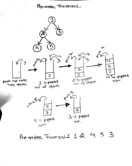
144.  Binary Tree Preorder Traversal (Difficulty: Medium)

To solve this question all we need to do is simply recall our magic spell. Let's understand the simulation really well since this is the basic template we will be using to solve the rest of the problems.

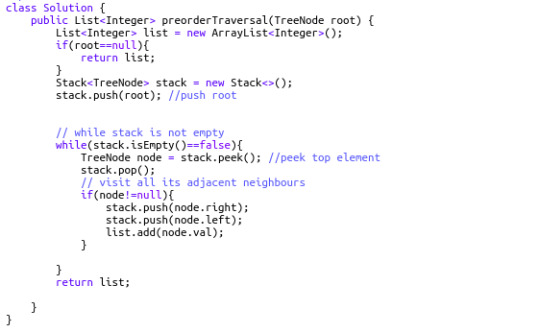
At first, we push the root node into the stack. While the stack is not empty, we pop it, and push its right and left child into the stack. As we pop the root node, we immediately put it into our result list. Thus, the first element in the result list is the root (hence the name, Pre-order). The next element to be popped from the stack will be the top element of the stack right now: the left child of root node. The process is continued in a similar manner until the whole graph has been traversed and all the node values of the binary tree enter into the resulting list.

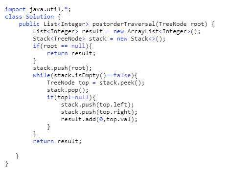
145. Binary Tree Postorder Traversal (Difficulty: Hard)

Pre-order traversal is root-left-right, and post-order is right-left-root. This means post order traversal is exactly the reverse of pre-order traversal. So one solution that might come to mind right now is simply reversing the resulting array of pre-order traversal. But think about it – that would cost O(n) time complexity to reverse it. A smarter solution is to copy and paste the exact code of the pre-order traversal, but put the result at the top of the linked list (index 0) at each iteration. It takes constant time to add an element to the head of a linked list. Cool, right?

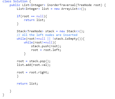
94. Binary Tree Inorder Traversal (Difficulty: Medium)

Our approach to solve this problem is similar to the previous problems. But here, we will visit everything on the left side of a node, print the node, and then visit everything on the right side of the node.

323. Number of Connected Components in an Undirected Graph (Difficulty: Medium)

Our approach here is to create a variable called ans that stores the number of connected components. First, we will initialize all vertices as unvisited. We will start from a node, and while carrying out DFS on that node (of course, using our magic spell), it will mark all the nodes connected to it as visited. The value of ans will be incremented by 1.

import java.util.ArrayList; import java.util.List; import java.util.Stack; public class NumberOfConnectedComponents { public static void main(String[] args){ int[][] edge = {{0,1}, {1,2},{3,4}}; int n = 5; System.out.println(connectedcount(n, edge)); } public static int connectedcount(int n, int[][] edges) { boolean[] visited = new boolean[n]; List[] adj = new List[n]; for(int i=0; i<adj.length; i++){ adj[i] = new ArrayList<Integer>(); } // create the adjacency list for(int[] e: edges){ int from = e[0]; int to = e[1]; adj[from].add(to); adj[to].add(from); } Stack<Integer> stack = new Stack<>(); int ans = 0; // ans = count of how many times DFS is carried out // this for loop through the entire graph for(int i = 0; i < n; i++){ // if a node is not visited if(!visited[i]){ ans++; //push it in the stack stack.push(i); while(!stack.empty()) { int current = stack.peek(); stack.pop(); //pop the node visited[current] = true; // mark the node as visited List<Integer> list1 = adj[current]; // push the connected components of the current node into stack for (int neighbours:list1) { if (!visited[neighbours]) { stack.push(neighbours); } } } } } return ans; } }

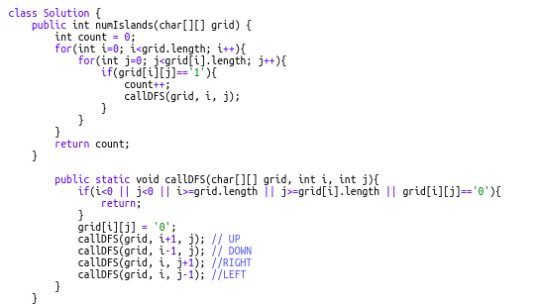
200. Number of Islands (Difficulty: Medium)

This falls under a general category of problems where we have to find the number of connected components, but the details are a bit tweaked. Instinctually, you might think that once we find a “1” we initiate a new component. We do a DFS from that cell in all 4 directions (up, down, right, left) and reach all 1’s connected to that cell. All these 1's connected to each other belong to the same group, and thus, our value of count is incremented by 1. We mark these cells of 1's as visited and move on to count other connected components.

547. Friend Circles (Difficulty: Medium)

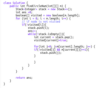
This also follows the same concept as finding the number of connected components. In this question, we have an NxN matrix but only N friends in total. Edges are directly given via the cells so we have to traverse a row to get the neighbors for a specific "friend". Notice that here, we use the same stack pattern as our previous problems.

That's all for today! I hope this has helped you understand DFS better and that you have enjoyed the tutorial. Please recommend this post if you think it may be useful for someone else!

[connective-environments-fall2019]

Reviews, Uploads, Website, and Readings

Read carefully the following (also uploaded in Google Drive here):

1. Reviews for Tuesday and deliverables for assignment 2

Each team will have 20 minutes of time (buzzer will sound at 10 minutes to give time for discussion). Presentation instructions:

1. Up to 10 slides documenting:

Design concept and inspirations

Drawings and axonometrics: front/top/back/side views and axonometric (isometric view – not perspective)

Axonometric exploded view showing all parts (see example)

Analysis/explanation of how the motor works including gear ration and, if possible, kinetic energy and torque

Fabrication and assembly process

Challenges faced and solutions

Assembly analysis including: liaison graph, adjacency matrix, assembly sequence.

Flexure joint details

A conclusion with what you learned from this experiment

Use a consistent color pallet for your drawings and presentation. Diagrams and line drawings should be monotone: only one color allowed; any number of shades. Use a consistent line weight and no more than two line types. Do not present screenshots from your Rhino screen. You will be judged not only on content but also on quality of your presentation.

2. A working prototype of your car demonstrating rigidity and robustness of your design

3. Live demonstration of how your car works. Your car will need to be able to independently move for at least two feet.

2. Google Drive Uploads (due Wednesday 12pm)

Slideshow (Powerpoint or PDF)

High-resolution, high-quality photos of the final prototype (white background)

High-resolution, high-quality photos of the the assembly process (white background)

All photos must be taken using white background. You can use the table in the Urban Synergetics Lab as a proper background for photos.

A high quality video on white background video demonstrating your car moving. The camera should be still (e.g. in a tripod – not using your hands) and the entire background should be white

High resolution photorealistic renderings

The laser cut sheet files in an appropriate replicate-able format (DXF, dwg, AI, Rhino, etc)

Rhino 3D model and Grasshopper file (if used) of your final car

PDFs of drawings and axonometrics

Photos of sketches, diagrams

3. Reviewers

Confirmed reviewers include: Greg Snyder, Mark Manack, Catty Dan Zhang. Full list of reviewers will be announced on Monday.

4. Website/Blog

Each week you are required to upload and document your work in the website. Web documentation is a requirement of the class – not an optional feature and you are being graded on that. Upload your documentations in the website by the end of the day tomorrow. I expect to see a narrative of your work. See instructions posted in the blog/website here.

5. Readings and homework for next Thursday

Come prepared to discuss in class the following (all readings have been uploaded in Google Drive week 3):

Required

Read chapters 1-10 (PDF) from Petzold, Charles. Code : The Hidden Language of Computer Hardware and Software. Book, Whole. Redmond, Wash., 2000.

Read chapters 2-5 (PDF) from Pierce, John R. Introduction to Information Theory: Symbols, Signals and Noise. Book, Whole, 2012.

Optional

Read chapters 1-2 (jpg files) from Stone, James V. Information Theory : A Tutorial Introduction. First Edition. Book, Whole. Sheffield, United Kingdom], 2015.

In teams of 3, discuss the following:

In your own words, what is Information Theory, what it allows us to know/do, and how? What is information entropy and why is it important in communication?

Discuss how Information Theory can be applied in designing/creating a communication system that is tangible (e.g. not relying on electricity or sound)? Can you imagine one? Bring examples or sketches.