#Running a Lasso Regression Analysis
Explore tagged Tumblr posts
Visit Tumblr Blog
Explore Tumblr blogs with no restrictions, modern design and the best experience.
Last Seen Tumblr Blogs


Fun Fact
In 2020, Tumblr had 29.4 million users in the US.
Text
Week 3: Peer-graded Assignment: Running a Lasso Regression Analysis
This assignment is intended for Coursera course "Machine Learning for Data Analysis by Wesleyan University”.
It is for " Week 3: Peer-graded Assignment: Running a Lasso Regression Analysis".
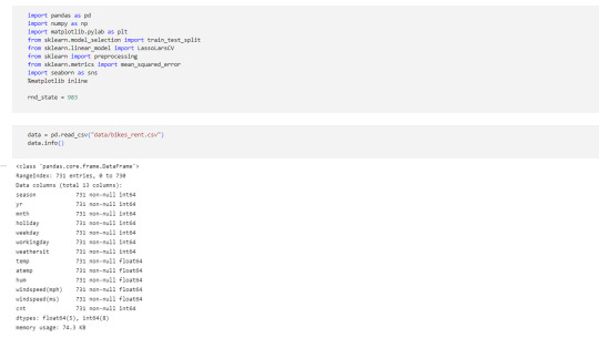
I am working on Lasso Regression Analysis in Python.
Syntax used to run Lasso Regression Analysis
Dataset description: hourly rental data spanning two years.
Dataset can be found at Kaggle
Features:
yr - year
mnth - month
season - 1 = spring, 2 = summer, 3 = fall, 4 = winter
holiday - whether the day is considered a holiday
workingday - whether the day is neither a weekend nor holiday
weathersit - 1: Clear, Few clouds, Partly cloudy, Partly cloudy
2: Mist + Cloudy, Mist + Broken clouds, Mist + Few clouds, Mist
3: Light Snow, Light Rain + Thunderstorm + Scattered clouds, Light Rain + Scattered clouds
4: Heavy Rain + Ice Pallets + Thunderstorm + Mist, Snow + Fog
temp - temperature in Celsius
atemp - "feels like" temperature in Celsius
hum - relative humidity
windspeed (mph) - wind speed, miles per hour
windspeed (ms) - wind speed, metre per second
Target:
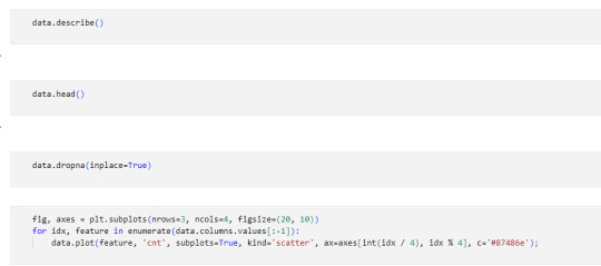
cnt - number of total rentals
Code used to run Lasso Regression Analysis
Corresponding Output
Interpretation
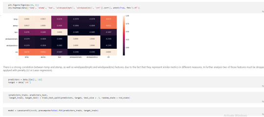
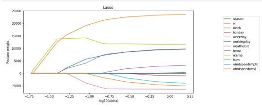
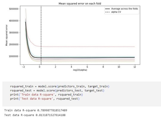
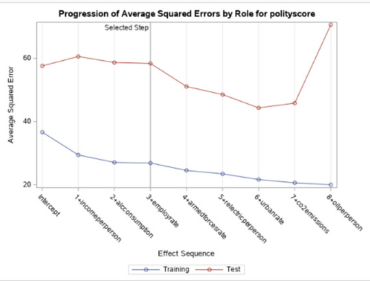
A lasso regression analysis was conducted to predict a number of total bikes rentals from a pool of 12 categorical and quantitative predictor variables that best predicted a quantitative response variable. Categorical predictors included weather condition and a series of 2 binary categorical variables for holiday and working day to improve interpretability of the selected model with fewer predictors. Quantitative predictor variables include year, month, temperature, humidity and wind speed. Data were randomly split into a training set that included 70% of the observations and a test set that included 30% of the observations. The least angle regression algorithm with k=10 fold cross validation was used to estimate the lasso regression model in the training set, and the model was validated using the test set. The change in the cross validation average (mean) squared error at each step was used to identify the best subset of predictor variables.
It tends to make coefficients to absolute zero as compared to Ridge which never sets the value of coefficient to absolute zero.
#Running a Lasso Regression Analysis#Machine Learning for Data Analysis#Wesleyan University#Coursera#Python#Week3
0 notes
Text


this week on megumi.fm ▸ media analysis brainrot
📋 Tasks
💻 Internship ↳ setup Linux system on alternate drive (this took me wayy more time than i anticipated) ✅ ↳ install yet more dependencies ✅ ↳ read up on protein folding and families + CATH and SCOP classifications ✅ ↳ download protein structure repositories ✅ ↳ run protein modeller pipeline ✅ ↳ read papers [3/3] ✅ ↳ set up a literature review tracker ✅ ↳ code for a program to parse PDB files to obtain protein seq ✅ 🎓 Uni Final Project our manuscript got a conditional acceptance!! ↳ revise and update manuscript and images according to changes mentioned ✅ 🩺 Radiomics Projects ↳ feature extraction from radiomics data using variance-based analysis ✅ ↳ setup LASSO regression (errors? look into this) 📧 Application-related ↳ collect internship experience letter ✅ ↳ collect degree transcripts ✅ ↳ request for referee report from my prof ✅
📅 Daily-s
🛌 consistent sleep [6/7] (binge watched too much TV and forgot about bed time booo) 💧 good water intake [5/7] (need to start carrying a bottle to work) 👟 exercise [4/7] (I really need to find time between work to move around)
Fun Stuff this week
🧁 met up with my bestfriends! we collected the mugs we painted last year and gifted them to each other! we also surprised one of our besties by showing up at her place. had waffles too ^=^ 📘 met up with another close friend for dinner! hung out at a bookshop after <3 🎮back at game videos: watched this critique on a time loop game called 12 minutes //then i switched up and got super obsessed with this game called The Beginner's Guide. I watched a video analysis on it, then went on to watch the entire gameplay, then read an article on the game's concept and what it means to analyze art and yeah. wow. after which I finally started playing the game with my best friend!! 📺 ongoing: Marry my Husband, Cherry Magic Th, Last Twilight 📺 binged: Taikan Yoho (aka My Personal Weatherman), Hometown Cha Cha Cha 📹 Horror Storytelling in the internet era
📻 This week's soundtrack
so. the Taikan Yoho brainrot was followed by me listening entirely to songs that evoked similar emotions to watching the main couple. personal fav emotions include a love that feels like you could die, a love that feels like losing yourself, a love that makes you feel like you could disappear, a love asking to be held, a love that reminds you that you're not alone, and a love that feels like a promise <3
---
[Jan 15 to 21; week 3/52 || I am having a blast at work ♡ I feel like I'm really learning and checking out a lot of cool stuff. That being said, I think I'm slacking when it comes to my daily routines in regards to my health. and I'm spending wayy too much time chained to my desk. maybe I'll request for an option to work from home so that I can cut on time taken on commute and spend that time exercising or walking
also. my obsession with tv shows is getting a bit. out of hand I think. not that it's particularly an issue? but I think I should switch back to my unread pile of books (or resume magpod) instead of spending my evenings on ki**a*ian. this could be unhealthy for my eyes in the long run, considering my work also involves staring at a screen all day. let's see.]
#52wktracker#studyblr#study blog#studyspo#stemblr#stem student#study goals#student life#college student#studying#stem studyblr#adhd studyblr#adhd student#study motivation#100 days of productivity#study inspo#study inspiration#gradblr#uniblr#studyinspo#sciblr#study aesthetic#study blr#study motivator#100 days of self discipline#100 days of studying#stem academia#bio student#100 dop#100dop
29 notes
·
View notes
Text
Running a Lasso Regression Analysis
Objective:
The code PROC GLMSELECT is used to perform LASSO (Least Absolute Shrinkage and Selection Operator) regression for feature selection on the dataset Gapminder. The objective is to determine which independent variables significantly predict incomeperperson. LASSO is used with the selection criterion C(p), which helps choose the best subset of predictors based on prediction error minimization.
Code:
PROC GLMSELECT DATA=Gapminder_Decision_Tree PLOTS(UNPACK)=ALL; MODEL incomeperperson = alcconsumption armedforcesrate breastcancerper100th co2emissions femaleemployrate hivrate internetuserate oilperperson polityscore relectricperperson suicideper100th employrate urbanrate lifeexpectancy / SELECTION=lasso(choose=CP) STATS=ALL; RUN;
Output:


Interpretation:
Model Selection:
The model selection stopped at Step 6 when the SBC criterion reached its minimum.
The selected model includes six predictors:
internetuserate
relectricperperson
lifeexpectancy
oilperperson
breastcancerper100th
co2emissions
The stopping criterion was based on Mallows' Cp, indicating a balance between model complexity and prediction accuracy.
Statistical Fit:
The final model explains 83.62% (R-Square = 0.8362) of the variance in income per person, indicating a strong model fit.
The adjusted R-Square (0.8161) is close to the R-Square, meaning the model generalizes well without overfitting.
The AIC (Akaike Information Criterion) and SBC (Schwarz Bayesian Criterion) values suggest that the selected model is optimal among tested models.
Variable Selection and Importance:
The LASSO selection process retained only six out of the fifteen variables, indicating these are the strongest predictors of incomeperperson.
The coefficient progression plot shows how predictors enter the model step by step.
relectricperperson has the largest coefficient, meaning it has the strongest influence on predicting incomeperperson.
Model Performance:
The Root Mean Square Error (RMSE) = 5451.29, showing the average deviation of predictions from actual values.
The Analysis of Variance (ANOVA) results confirm that the selected predictors significantly improve model performance.
0 notes
Text
OOL Attacker - Running a Lasso Regression Analysis
For this project it was used the Outlook on Life Surveys. "The purpose of the 2012 Outlook Surveys were to study political and social attitudes in the United States. The specific purpose of the survey is to consider the ways in which social class, ethnicity, marital status, feminism, religiosity, political orientation, and cultural beliefs or stereotypes influence opinion and behavior." - Outlook
Was necessary the removal of some rows containing text (for confidentiality purposes) before the dorpna() function.
This is my full code:
import pandas as pd import numpy as np import matplotlib.pylab as plt from sklearn.model_selection import train_test_split from sklearn.linear_model import LassoLarsCV from sklearn import preprocessing import time #Load the dataset data = pd.read_csv(r"PATHHHH") #upper-case all DataFrame column names data.columns = map(str.upper, data.columns) # Data Management data_clean = data.select_dtypes(include=['number']) data_clean = data_clean.dropna() print(data_clean.describe()) print(data_clean.dtypes) #Split into training and testing sets headers = list(data_clean.columns) headers.remove("PPNET") predvar = data_clean[headers] target = data_clean.PPNET predictors=predvar.copy() for header in headers: predictors[header] = preprocessing.scale(predictors[header].astype('float64')) # split data into train and test sets pred_train, pred_test, tar_train, tar_test = train_test_split(predictors, target, test_size=.3, random_state=123) # specify the lasso regression model model=LassoLarsCV(cv=10, precompute=False).fit(pred_train,tar_train) #Display both categories by coefs pd.set_option('display.max_rows', None) table_catimp=pd.DataFrame({'cat': predictors.columns, 'coef': abs(model.coef_)}) print(table_catimp) non_zero_count = (table_catimp['coef'] != 0).sum() zero_count = table_catimp.shape[0] - non_zero_count print(f"Number of non-zero coefficients: {non_zero_count}") print(f"Number of zero coefficients: {zero_count}") #Display top 5 categories by coefs top_5_rows = table_catimp.nlargest(10, 'coef') print(top_5_rows.to_string(index=False)) # plot coefficient progression m_log_alphas = -np.log10(model.alphas_) ax = plt.gca() plt.plot(m_log_alphas, model.coef_path_.T) plt.axvline(-np.log10(model.alpha_), linestyle='--', color='k', label='alpha CV') plt.ylabel('Regression Coefficients') plt.xlabel('-log(alpha)') plt.title('Regression Coefficients Progression for Lasso Paths') # plot mean square error for each fold m_log_alphascv = -np.log10(model.cv_alphas_) plt.figure() plt.plot(m_log_alphascv, model.mse_path_, ':') plt.plot(m_log_alphascv, model.mse_path_.mean(axis=-1), 'k', label='Average across the folds', linewidth=2) plt.axvline(-np.log10(model.alpha_), linestyle='--', color='k', label='alpha CV') plt.legend() plt.xlabel('-log(alpha)') plt.ylabel('Mean squared error') plt.title('Mean squared error on each fold') # MSE from training and test data from sklearn.metrics import mean_squared_error train_error = mean_squared_error(tar_train, model.predict(pred_train)) test_error = mean_squared_error(tar_test, model.predict(pred_test)) print ('training data MSE') print(train_error) print ('test data MSE') print(test_error) # R-square from training and test data rsquared_train=model.score(pred_train,tar_train) rsquared_test=model.score(pred_test,tar_test) print ('training data R-square') print(rsquared_train) print ('test data R-square') print(rsquared_test) plt.show()
Output:
Number of non-zero coefficients: 54 Number of zero coefficients: 186 training data MSE: 0.11867468892072082 test data MSE: 0.1458371486851879 training data R-square: 0.29967753231880834 test data R-square: 0.18204209521525183
Top 10 coefs:
PPINCIMP 0.097772 W1_WEIGHT3 0.061791 W1_P21 0.048740 W1_E1 0.027003 W1_CASEID 0.026709 PPHHSIZE 0.026055 PPAGECT4 0.022809 W1_Q1_B 0.021630 W1_P16E 0.020672 W1_E63_C 0.020205
Conclusions:
While the test error is slightly higher than the training error, the difference is not extreme, which is a positive sign that the model generalizes reasonably well.
Also in another note, the drop in R-square between training and test sets suggests the model may be overfitting slightly or that the predictors do not fully explain the response variable's behavior.
In the attachments I present the Regression coefficients, allowing to verify which features or characteristics are the most relevant for this model. Both PPINCIMP and W1_WEIGHT3 have the biggest weight. In the second attachment we can select the optimal alpha, the vertical dashed line indicates the optimal value of alpha.


The program successfully identified a subset of 54 predictors from 240 variables that are most strongly associated with the response variable. The moderate R-square values suggest room for improvement in the model's explanatory power. However, the close alignment between training and test MSE indicates reasonable generalization.
0 notes
Text
Title: Lasso Regression Analysis with k-Fold Cross Validation for Variable Selection
1. Introduction to Lasso Regression
Lasso Regression is a statistical method for shrinkage and variable selection in linear regression models. The goal of Lasso is to shrink the coefficients of some variables to zero, effectively eliminating these variables from the model. This results in a model that uses only the most significant predictors for forecasting the response variable.
2. Steps for Performing the Analysis:
1. Data Loading and Preparation:
In this case, we used synthetic data generated by the make_regression function from sklearn, which provides dummy data for the purpose of analysis.
2. Data Splitting:
Since the dataset is small, there was no need to split it into training and testing sets. We used k-Fold Cross Validation to assess the model's performance.
3. Lasso Model Creation:
We defined a Lasso model with the alpha parameter to control the strength of the shrinkage.
4. Performing Cross Validation (Cross-Validation):
We used 5 folds (k=5) for KFold Cross Validation to evaluate the model's performance.
3. The Code Used:

4. Model Output:
When the code is run, the following outputs are obtained (values may vary based on the data):
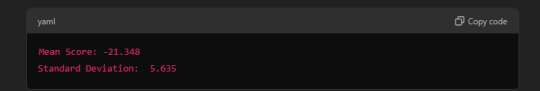
Mean Score: This is the average negative mean squared error (MSE) across the cross-validation folds. The more negative this value, the better the model performs in terms of prediction accuracy.
Standard Deviation: This shows the variation in the model's performance across different folds.
5. Analysis:
From the cross-validation results, we observe that the model gives an average negative mean squared error (MSE) of -21.348, which indicates that the model is performing reasonably well.
Lasso has effectively shrunk some coefficients to zero, thus helping to select the most significant variables while removing unnecessary ones.
6. Summary:
We used Lasso Regression with k-Fold Cross Validation to select the most important predictors from a larger set of variables.
Through this process, variables with coefficients shrunk to zero were excluded from the model, and the remaining significant variables were chosen.
0 notes
Text
Running a Lasso Regression Analysis
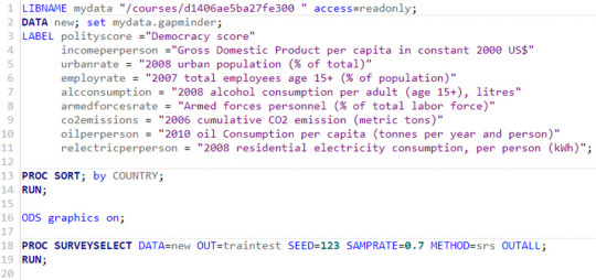
My task today is to test a running a lasso regression analysis. A lasso regression analysis was conducted to identify a subset of variables from a pool of 8 quantitative predictor variables that best predicted a quantitative response variable measuring country democracy score. A lasso regression analysis was conducted to identify a subset of variables from a pool of 8 quantitative predictor variables that best predicted a quantitative response variable measuring country democracy score.
Quantitative predictor variables include:
income per person - Gross Domestic Product per capita in constant 2000 US$;
urban rate - 2008 urban population (% of total);
employ rate - 2007 total employees age 15+ (% of population);
alcohol consumption - 2008 alcohol consumption per adult (age 15+), litres;
armed forces rate - Armed forces personnel (% of total labor force);
CO2 emissions - 2006 cumulative CO2 emission (metric tons);
oil per person - 2010 oil Consumption per capita (tonnes per year and person);
electric per person - 2008 residential electricity consumption, per person (kWh).
All predictor variables were standardized to have a mean of zero and a standard deviation of one.
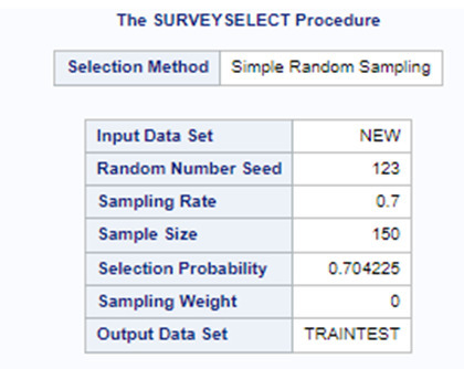
To run a lasso regression analysis, I wrote the following SAS code.
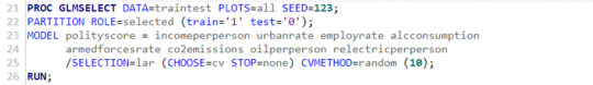
Data were randomly split into a training set that included 70% of the observations (N=37) and a test set that included 30% of the observations (N=23). The least angle regression algorithm with k=10 fold cross validation was used to estimate the lasso regression model in the training set, and the model was validated using the test set. The change in the cross validation average (mean) squared error at each step was used to identify the best subset of predictor variables.
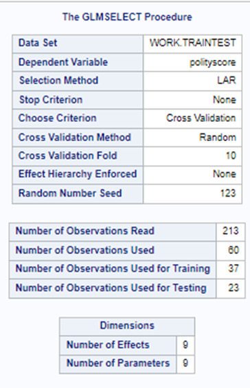
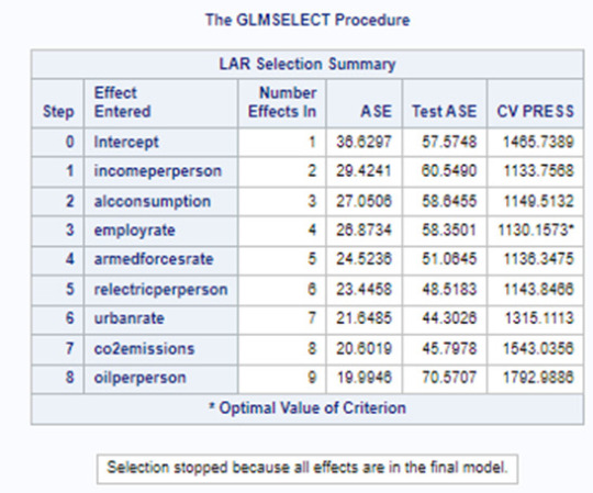
Of the 9 predictor variables, 3 were retained in the selected model. During the estimation process, polity scores were most strongly associated with income per person followed by alcohol consumption and employment rate. Income per person and alcohol consumption was positively associated with the polity score and employment rate was negatively associated with the polity score.
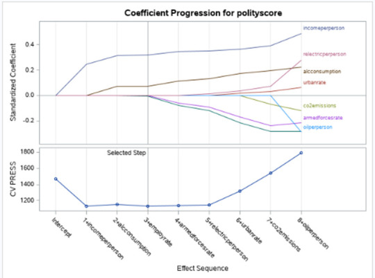
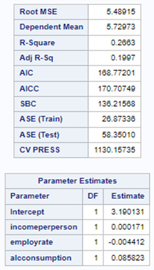
In the following screenshot, we can see the values of the coefficients in the linear regression equation. Thus, the beta sub zero is 3.1901, beta sub one equals 0.0002, beta sub two – (-0.0044), beta sub three – 0.0858. Now we know that our equation for the multiple regression line is:
polity score = 3.1901 + 0.0002 * income per person – 0.0044* employ rate + 0.0858* alcohol consumption.
0 notes
Text
Capstone Milestone Assignment 2: Methods
Full Code: https://github.com/sonarsujit/MSC-Data-Science_Project/blob/main/capstoneprojectcode.py
Methods
1. Sample: The data for this study was drawn from the World Bank's global dataset, which includes comprehensive economic and health indicators from various countries across the world. The final sample consists of N = 248 countries, and I am only looking at the 2012 data for this sample data.
Sample Description: The sample includes countries from various income levels, regions, and development stages. It encompasses both high-income countries with advanced healthcare systems and low-income countries where access to healthcare services might be limited. The sample is diverse in terms of geographic distribution, economic conditions, and public health outcomes, providing a comprehensive view of global health disparities.
2. Measures: The given dataset has 86 variables and form the perspective of answering the research question, I focused on life expectancy and access to healthcare services. The objective is to look into these features statistically and narrow down to relevant and important features that will align to my research problem.
Here's a breakdown of the selected features and how they relate to my research:
Healthcare Access and Infrastructure: Access to electricity, Access to non-solid fuel,Fixed broadband subscriptions, Improved sanitation facilities, Improved water source, Internet users
Key Health and Demographic Indicators: Adolescent fertility rate, Birth rate, Cause of death by communicable diseases and maternal/prenatal/nutrition conditions, Fertility rate, Mortality rate, infant , Mortality rate, neonatal , Mortality rate, under-5, Population ages 0-14 ,Urban population growth
Socioeconomic Factors: Population ages 65 and above, Survival to age 65, female, Survival to age 65, male, Adjusted net national income per capita, Automated teller machines (ATMs), GDP per capita, Health expenditure per capita, Population ages 15-64, Urban population.
Variable Management:
The Life Expectancy variable was used as a continuous variable in the analysis.
All the independent variables were also used as continuous variables.
Out of the 84 in quantitative independent variables, I found that the above 26 features closely describe the health access and infrastructure, key health and demographic indicators and socioeconomic factors based on the literature review.
I run the Lasso regression to get insights on features that will align more closely with my research question
Table1: Lasso regression to find important features that support my research question.

Based on the result from lasso regression, I finalized 8 predictor variables which I believe will potentially help me answer my research question.
To further support the selection of these 8 features, I run Correlation Analysis for these 8 features and found to have both positive and negative correlations with the target variable (Life Expectancy at Birth, Total (Years))
Table 2: Pearson Correlation values and relative p values

The inclusion of both positive and negative correlations provides a balanced view of the factors affecting life expectancy, making these features suitable for your analysis.
Incorporating these variables should allow us to capture the multifaceted relationship between healthcare access and life expectancy across different countries, and effectively address our research question.
Analyses:
The primary goal of the analysis was to explore and understand the factors that influence life expectancy across different countries. This involved using Lasso regression for feature selection and Pearson correlation for assessing the strength of relationships between life expectancy and various predictor variables.
The Lasso model revealed that factors such as survival rates to age 65, health expenditure, broadband access, and mortality rate under 5 were the most significant predictors of life expectancy.
The mean squared error (MSE) = 1.2686 of the model was calculated to assess its predictive performance.
Survival to age 65 (both male and female) had strong positive correlations with life expectancy, indicating that populations with higher survival rates to age 65 tend to have higher overall life expectancy.
Health expenditure per capita showed a moderate positive correlation, suggesting that countries investing more in healthcare tend to have longer life expectancy.
Mortality rate, under-5 (per 1,000) had a strong negative correlation with life expectancy, highlighting that higher child mortality rates are associated with lower life expectancy.
Rural population (% of total) had a negative correlation, indicating that countries with a higher percentage of rural populations might face challenges that reduce life expectancy.
0 notes
Text
Running a Lasso Regression Analysis to identify a subset of variables that best predicted the alcohol drinking behavior of individuals
A lasso regression analysis is performed to detect a subgroup of variables from a set of 23 categorical and quantitative predictor variables in the Nesarc Wave 1 dataset which best predicted a quantitative response variable assessing the alcohol drinking behaviour of individuals 18 years and older in terms of number of any alcohol drunk per month.
Categorical predictors include a series of 5 binary categorical variables for ethnicity (Hispanic, White, Black, Native American and Asian) to improve interpretability of the selected model with fewer predictors.
Other binary categorical predictors are related to substance consumption, and in particular to the fact whether or not individuals are lifetime opioids, cannabis, cocaine, sedatives, tranquilizers consumers, as well as suffer from depression.
About dependencies, other binary categorical variables are those regarding if individuals
are lifetime affected by nicotine dependency,
abuse lifetime of alcohol
or not.
Quantitative predictor variables include age when the aforementioned substances have been taken for the first time, the usual frequency of cigarettes and of any alcohol drunk per month, the number of cigarettes smoked per month.
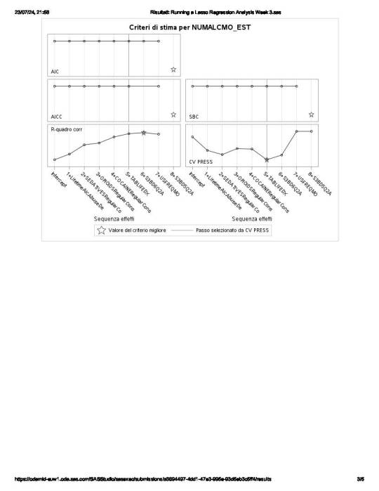
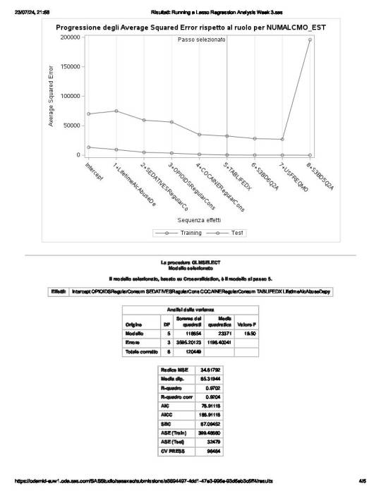
In a nutshell, looking at the SAS output,
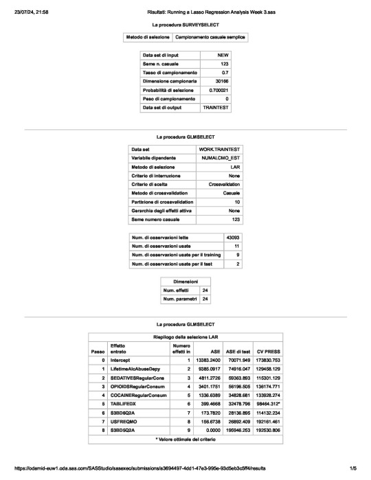
the survey select procedure, used to split the observations in the dataset into training and test data, shows that the sample size is 30,166.
the so-called “NUMALCMO_EST” dependent variable - number of any alcohol drunk per month - along with the selection method used, are being displayed, together with information such as
the choice of a cross validation criteria as criterion for choosing the best model, with K equals 10-fold cross validation,
the random assignments of observations to the folds
the total number of observations in the data set are 43093 and the number of observations used for training and testing the statistical models are 11, where 9 are for training and 2 for testing
the number of parameters to be estimated is 24 for the intercept plus the 23 predictors.
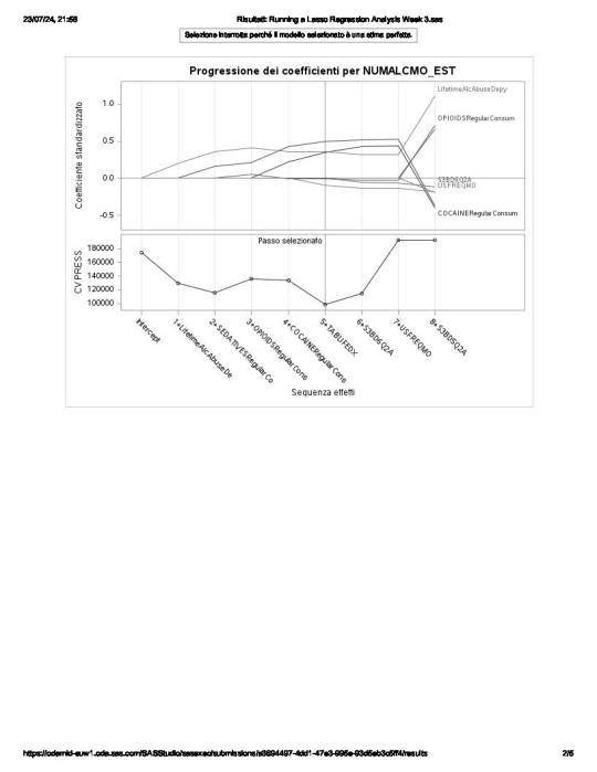
of the 23 predictor variables, 8 have been maintained in the selected model:
LifetimeAlcAbuseDepy - alcohol abuse / dependence both in last 12 months and prior to the last 12 months
and
OPIOIDSRegularConsumer – used opioids both in the last 12 months and prior to the last 12 months
have the largest regression coefficient, followed by COCAINERegularConsum behaviour.
LifetimeAlcAbuseDepy and OPIOIDSRegularConsum are positively associated with the response variable, while COCAINERegularConsum is negatively associated with NUMALCMO_EST.
Other predictors associated with lower number of any alcohol drunk per month are S3BD6Q2A – “age first used cocaine or crack” and USEFREQMO – “usual frequency of cigarettes smoked per month”.
These 8 variables accounted for 33.6% of the variance in the number of any alcohol drunk per month response variable.
Hereunder the SAS code used to generate the present analysis and the plots on which the above described results are depicted
PROC IMPORT DATAFILE ='/home/u63783903/my_courses/nesarc_pds.csv' OUT = imported REPLACE; RUN; DATA new; set imported;
/* lib name statement and data step to call in the NESARC data set for the purpose of growing decision trees*/
LABEL MAJORDEPLIFE = "MAJOR DEPRESSION - LIFETIME" ETHRACE2A = "IMPUTED RACE/ETHNICITY" WhiteGroup = "White, Not Hispanic or Latino" BlackGroup = "Black, Not Hispanic or Latino" NamericaGroup = "American Indian/Alaska Native, Not Hispanic or Latino" AsianGroup = "Asian/Native Hawaiian/Pacific Islander, Not Hispanic or Latino" HispanicGroup = "Hispanic or Latino" S3BD3Q2B = "USED OPIOIDS IN THE LAST 12 MONTHS/PRIOR TO LAST 12 MONTHS/BOTH TIME PERIODS" OPIOIDSRegularConsumer = "USED OPIOIDS both IN THE LAST 12 MONTHS AND PRIOR TO LAST 12 MONTHS" S3BD3Q2A = "AGE FIRST USED OPIOIDS" S3BD5Q2B = "USED CANNABIS IN THE LAST 12 MONTHS/PRIOR TO LAST 12 MONTHS/BOTH TIME PERIODS" CANNABISRegularConsumer = "USED CANNABIS both IN THE LAST 12 MONTHS AND PRIOR TO LAST 12 MONTHS" S3BD5Q2A = "AGE FIRST USED CANNABIS" S3BD1Q2B = "USED SEDATIVES IN THE LAST 12 MONTHS/PRIOR TO LAST 12 MONTHS/BOTH TIME PERIODS" SEDATIVESRegularConsumer = "USED SEDATIVES both IN THE LAST 12 MONTHS/PRIOR TO LAST 12 MONTHS" S3BD1Q2A = "AGE FIRST USED SEDATIVES" S3BD2Q2B = "USED TRANQUILIZERS IN THE LAST 12 MONTHS/PRIOR TO LAST 12 MONTHS/BOTH TIME PERIODS" TRANQUILIZERSRegularConsumer = "USED TRANQUILIZERS both IN THE LAST 12 MONTHS AND PRIOR TO LAST 12 MONTHS" S3BD2Q2A = "AGE FIRST USED TRANQUILIZERS" S3BD6Q2B = "USED COCAINE OR CRACK IN THE LAST 12 MONTHS/PRIOR TO LAST 12 MONTHS/BOTH TIME PERIODS" COCAINERegularConsumer = "USED COCAINE both IN THE LAST 12 MONTHS AND PRIOR TO LAST 12 MONTHS" S3BD6Q2A = "AGE FIRST USED COCAINE OR CRACK" TABLIFEDX = "NICOTINE DEPENDENCE - LIFETIME" ALCABDEP12DX = "ALCOHOL ABUSE/DEPENDENCE IN LAST 12 MONTHS" ALCABDEPP12DX = "ALCOHOL ABUSE/DEPENDENCE PRIOR TO THE LAST 12 MONTHS" LifetimeAlcAbuseDepy = "ALCOHOL ABUSE/DEPENDENCE both IN LAST 12 MONTHS and PRIOR TO THE LAST 12 MONTHS" S3AQ3C1 = "USUAL QUANTITY WHEN SMOKED CIGARETTES" S3AQ3B1 = "USUAL FREQUENCY WHEN SMOKED CIGARETTES" USFREQMO = "usual frequency of cigarettes smoked per month" NUMCIGMO_EST= "NUMBER OF cigarettes smoked per month" S2AQ8A = "HOW OFTEN DRANK ANY ALCOHOL IN LAST 12 MONTHS" S2AQ8B = "NUMBER OF DRINKS OF ANY ALCOHOL USUALLY CONSUMED ON DAYS WHEN DRANK ALCOHOL IN LAST 12 MONTHS" USFREQALCMO = "usual frequency of any alcohol drunk per month" NUMALCMO_EST = "NUMBER OF ANY ALCOHOL drunk per month" S3BD1Q2E = "HOW OFTEN USED SEDATIVES WHEN USING THE MOST" USFREQSEDATIVESMO = "usual frequency of any alcohol drunk per month" S1Q1F = "BORN IN UNITED STATES"
if cmiss(of _all_) then delete; /* delete observations with missing data on any of the variables in the NESARC dataset */
if ETHRACE2A=1 then WhiteGroup=1; else WhiteGroup=0; /* creation of a variable for white ethnicity coded for 0 for non white ethnicity and 1 for white ethnicity */
if ETHRACE2A=2 then BlackGroup=1; else BlackGroup=0; /* creation of a variable for black ethnicity coded for 0 for non black ethnicity and 1 for black ethnicity */
if ETHRACE2A=3 then NamericaGroup=1; else NamericaGrouGroup=0; /* same for native american ethnicity*/
if ETHRACE2A=4 then AsianGroup=1; else AsianGroup=0; /* same for asian ethnicity */
if ETHRACE2A=5 then HispanicGroup=1; else HispanicGroup=0; /* same for hispanic ethnicity */
if S3BD3Q2B = 9 then S3BD3Q2B = .; /* unknown observations set to missing data wrt usage of OPIOIDS IN THE LAST 12 MONTHS/PRIOR TO LAST 12 MONTHS/BOTH TIME PERIODS */
if S3BD3Q2B = 3 then OPIOIDSRegularConsumer = 1; if S3BD3Q2B = 1 or S3BD3Q2B = 2 then OPIOIDSRegularConsumer = 0; if S3BD3Q2B = . then OPIOIDSRegularConsumer = .; /* creation of a group variable where lifetime opioids consumers are coded to 1 and 0 for non lifetime opioids consumers */
if S3BD3Q2A = 99 then S3BD3Q2A = . ; /* unknown observations set to missing data wrt AGE FIRST USED OPIOIDS */
if S3BD5Q2B = 9 then S3BD5Q2B = .; /* unknown observations set to missing data wrt usage of CANNABIS IN THE LAST 12 MONTHS/PRIOR TO LAST 12 MONTHS/BOTH TIME PERIODS */
if S3BD5Q2B = 3 then CANNABISRegularConsumer = 1; if S3BD5Q2B = 1 or S3BD5Q2B = 2 then CANNABISRegularConsumer = 0; if S3BD5Q2B = . then CANNABISRegularConsumer = .; /* creation of a group variable where lifetime cannabis consumers are coded to 1 and 0 for non lifetime cannabis consumers */
if S3BD5Q2A = 99 then S3BD5Q2A = . ; /* unknown observations set to missing data wrt AGE FIRST USED CANNABIS */
if S3BD1Q2B = 9 then S3BD1Q2B = .; /* unknown observations set to missing data wrt usage of SEDATIVES IN THE LAST 12 MONTHS/PRIOR TO LAST 12 MONTHS/BOTH TIME PERIODS */
if S3BD1Q2B = 3 then SEDATIVESRegularConsumer = 1; if S3BD1Q2B = 1 or S3BD1Q2B = 2 then SEDATIVESRegularConsumer = 0; if S3BD1Q2B = . then SEDATIVESRegularConsumer = .; /* creation of a group variable where lifetime sedatives consumers are coded to 1 and 0 for non lifetime sedatives consumers */
if S3BD1Q2A = 99 then S3BD1Q2A = . ; /* unknown observations set to missing data wrt AGE FIRST USED sedatives */
if S3BD2Q2B = 9 then S3BD1Q2B = .; /* unknown observations set to missing data wrt usage of TRANQUILIZERS IN THE LAST 12 MONTHS/PRIOR TO LAST 12 MONTHS/BOTH TIME PERIODS */
if S3BD2Q2B = 3 then TRANQUILIZERSRegularConsumer = 1; if S3BD2Q2B = 1 or S3BD2Q2B = 2 then TRANQUILIZERSRegularConsumer = 0; if S3BD2Q2B = . then TRANQUILIZERSRegularConsumer = .; /* creation of a group variable where lifetime TRANQUILIZERS consumers are coded to 1 and 0 for non lifetime TRANQUILIZERS consumers */
if S3BD2Q2A = 99 then S3BD2Q2A = . ; /* unknown observations set to missing data wrt AGE FIRST USED TRANQUILIZERS */
if S3BD6Q2A = 9 then S3BD6Q2A = .; /* unknown observations set to missing data wrt usage of COCAINE IN THE LAST 12 MONTHS/PRIOR TO LAST 12 MONTHS/BOTH TIME PERIODS */
if S3BD6Q2B = 3 then COCAINERegularConsumer = 1; if S3BD6Q2B = 1 or S3BD6Q2B = 2 then COCAINERegularConsumer = 0; if S3BD6Q2B = . then COCAINERegularConsumer = .; /* creation of a group variable where lifetime COCAINE consumers are coded to 1 and 0 for non lifetime COCAINE consumers */
if S3BD6Q2A = 99 then S3BD2Q2A = . ; /* unknown observations set to missing data wrt AGE FIRST USED COCAINE */
if ALCABDEP12DX = 3 and ALCABDEPP12DX = 3 then LifetimeAlcAbuseDepy =1; else LifetimeAlcAbuseDepy = 0; /* creation of a group variable where consumers with lifetime alcohol abuse and dependence are coded to 1 and 0 for consumers with no lifetime alcohol abuse and dependence */
if S3AQ3C1=99 THEN S3AQ3C1=.;
IF S3AQ3B1=9 THEN SS3AQ3B1=.;
IF S3AQ3B1=1 THEN USFREQMO=30; ELSE IF S3AQ3B1=2 THEN USFREQMO=22; ELSE IF S3AQ3B1=3 THEN USFREQMO=14; ELSE IF S3AQ3B1=4 THEN USFREQMO=5; ELSE IF S3AQ3B1=5 THEN USFREQMO=2.5; ELSE IF S3AQ3B1=6 THEN USFREQMO=1; /* usual frequency of smoking per month */
NUMCIGMO_EST=USFREQMO*S3AQ3C1; /* number of cigarettes smoked per month */
if S2AQ8A=99 THEN S2AQ8A=.;
if S2AQ8B = 99 then S2AQ8B = . ;
IF S2AQ8A=1 THEN USFREQALCMO=30; ELSE IF S2AQ8A=2 THEN USFREQALCMO=30; ELSE IF S2AQ8A=3 THEN USFREQALCMO=14; ELSE IF S2AQ8A=4 THEN USFREQALCMO=8; ELSE IF S2AQ8A=5 THEN USFREQALCMO=4; ELSE IF S2AQ8A=6 THEN USFREQALCMO=2.5; ELSE IF S2AQ8A=7 THEN USFREQALCMO=1; ELSE IF S2AQ8A=8 THEN USFREQALCMO=0.75; ELSE IF S2AQ8A=9 THEN USFREQALCMO=0.375; ELSE IF S2AQ8A=10 THEN USFREQALCMO=0.125; /* usual frquency of alcohol drinking per month */
NUMALCMO_EST=USFREQALCMO*S2AQ8B; /* number of any alcohol drunk per month */
if S3BD1Q2E=99 THEN S3BD1Q2E=.;
IF S3BD1Q2E=1 THEN USFREQSEDATIVESMO=30; ELSE IF S3BD1Q2E=2 THEN USFREQSEDATIVESMO=30; ELSE IF S3BD1Q2E=3 THEN USFREQSEDATIVESMO=14; ELSE IF S3BD1Q2E=4 THEN USFREQSEDATIVESMO=6; ELSE IF S3BD1Q2E=5 THEN USFREQSEDATIVESMO=2.5; ELSE IF S3BD1Q2E=6 THEN USFREQSEDATIVESMO=1; ELSE IF S3BD1Q2E=7 THEN USFREQSEDATIVESMO=0.75; ELSE IF S3BD1Q2E=8 THEN USFREQSEDATIVESMO=0.375; ELSE IF S3BD1Q2E=9 THEN USFREQSEDATIVESMO=0.17; ELSE IF S3BD1Q2E=10 THEN USFREQSEDATIVESMO=0.083; /* usual frequency of seadtives assumption per month */
run;
ods graphics on; /* ODS graphics turned on to manage the output and displays in HTML */
proc surveyselect data=new out=traintest seed = 123 samprate=0.7 method=srs outall; run;
/* split data randomly into training data consisting of 70% of the total observations () test dataset consisting of the other 30% of the observations respectively)*/ /* data=new specifies the name of the managed input data set */ /* out equals the name of the randomly split output dataset, called traintest */ /* seed option to specify a random number seed to ensure that the data are randomly split the same way if the code being run again */ /* samprate command split the input data set so that 70% of the observations are being designated as training observations (the remaining 30% are being designated as test observations respectively) */ /* method=srs specifies that the data are to be split using simple random sampling */ /* outall option includes, both the training and test observations in a single output dataset which has a new variable called "selected", to indicate if an observation belongs to the training set, or the test set */
proc glmselect data=traintest plots=all seed=123; partition ROLE=selected(train='1' test='0'); /* glmselect procedure to test the lasso multiple regression w/ Least Angled Regression algorithm k=10 fold validation glmselect procedure standardize the predictor variables, so that they all have a mean equal to 0 and a standard deviation equal to 1, which places them all on the same scale data=traintest to use the randomly split dataset plots=all option to require that all plots associated w/ the lasso regression being printed seed option to allow to specify a random number seed, being used in the cross-validation process partition command to assign each observation a role, based on the variable called selected, indicating if the observation is a training or test observation. Observations with a value of 1 on the selected variable are assigned the role of training observation (observations with a value of 0, are assigned the role of test observation respectively) */
model NUMALCMO_EST = MAJORDEPLIFE WhiteGroup BlackGroup NamericaGroup AsianGroup HispanicGroup OPIOIDSRegularConsumer S3BD3Q2A CANNABISRegularConsumer S3BD5Q2A SEDATIVESRegularConsumer S3BD1Q2A TRANQUILIZERSRegularConsumer S3BD2Q2A COCAINERegularConsumer S3BD6Q2A TABLIFEDX LifetimeAlcAbuseDepy USFREQMO NUMCIGMO_EST USFREQALCMO S3BD1Q2E USFREQSEDATIVESMO/selection=lar(choose=cv stop=none) cvmethod=random(10); /* model command to specify the regression model for which the response variable, NUMALCMO_EST, is equal to the list of the 14 candidate predictor variables */ /* selection option to tell which method to use to compute the parameters for variable selection */ /*Least Angled Regression algorithm is being used */ /* choose=cv option to use cross validation for choosing the final statistical model */ /* stop=none to guarantee the model doesn't stop running until each of the candidate predictor variables is being tested */ /* cvmethod=random(10) to specify a K-fold cross-validation method with ten randomly selected folds is being used */ run;

0 notes
Text
Lasso Regression Analysis
To run a Lasso regression analysis, you will use a programming language like Python with appropriate libraries. Here’s a guide to help you complete this assignment:### Step 1: Prepare Your DataEnsure your data is ready for analysis, including explanatory variables and a quantitative response variable.###
Step 2: Import Necessary LibrariesFor this example, I’ll use Python and the `scikit-learn` library.#### Python```pythonimport pandas as pdimport numpy as npfrom sklearn.model_selection import train_test_split, KFold, cross_val_scorefrom sklearn.linear_model import LassoCVfrom sklearn.metrics import mean_squared_errorimport matplotlib.pyplot as plt```###
Step 3: Load Your Data```python# Load your datasetdata = pd.read_csv('your_dataset.csv')# Define explanatory variables (X) and response variable (y)X = data.drop('target_variable', axis=1)y = data['target_variable']```###
Step 4: Set Up k-Fold Cross-Validation```python# Define k-fold cross-validationkf = KFold(n_splits=5, shuffle=True, random_state=42)```###
Step 5: Train the Lasso Regression Model with Cross-Validation```python# Initialize and train the LassoCV modellasso = LassoCV(cv=kf, random_state=42)lasso.fit(X, y)```###
Step 6: Evaluate the Model```python# Evaluate the model's performancemse = mean_squared_error(y, lasso.predict(X))print(f'Mean Squared Error: {mse:.2f}')# Coefficients of the modelcoefficients = pd.Series(lasso.coef_, index=X.columns)print('Lasso Coefficients:')print(coefficients)```###
Step 7: Visualize the Coefficients```python# Plot non-zero coefficientsplt.figure(figsize=(10,6))coefficients[coefficients != 0].plot(kind='barh')plt.title('Lasso Regression Coefficients')plt.show()```### InterpretationAfter running the above code, you'll have the output from your model, including the mean squared error, coefficients of the model, and a plot of the non-zero coefficients. Here’s an example of how you might interpret the results:- **Mean Squared Error (MSE)**: This metric shows the average squared difference between the observed actual outcomes and the outcomes predicted by the model. A lower MSE indicates better model performance.- **Lasso Coefficients**: The coefficients show the importance of each feature in the model. Features with coefficients equal to zero are excluded from the model, while those with non-zero coefficients are retained. The bar plot visualizes these non-zero coefficients, indicating which features are most strongly associated with the response variable.
### Blog Entry SubmissionFor your blog entry, include:-
The code used to run the Lasso regression (as shown above).- Screenshots or text of the output (MSE, coefficients, and coefficient plot).- A brief interpretation of the results.If your dataset is small and you decide not to split it into training and test sets, provide a rationale for this decision in your summary. Ensure the content is clear and understandable for peers who may not be experts in the field. This will help them effectively assess your work.
0 notes
Text
Run a lasso regression analysis
To run a Lasso regression analysis, you will use a programming language like Python with appropriate libraries. Here’s a guide to help you complete this assignment:
Step 1: Prepare Your Data
Ensure your data is ready for analysis, including explanatory variables and a quantitative response variable.
Step 2: Import Necessary Libraries
For this example, I’ll use Python and the scikit-learn library.
Python
import pandas as pd import numpy as np from sklearn.model_selection import train_test_split, KFold, cross_val_score from sklearn.linear_model import LassoCV from sklearn.metrics import mean_squared_error import matplotlib.pyplot as plt
Step 3: Load Your Data
# Load your dataset data = pd.read_csv('your_dataset.csv') # Define explanatory variables (X) and response variable (y) X = data.drop('target_variable', axis=1) y = data['target_variable']
Step 4: Set Up k-Fold Cross-Validation
# Define k-fold cross-validation kf = KFold(n_splits=5, shuffle=True, random_state=42)
Step 5: Train the Lasso Regression Model with Cross-Validation
# Initialize and train the LassoCV model lasso = LassoCV(cv=kf, random_state=42) lasso.fit(X, y)
Step 6: Evaluate the Model
# Evaluate the model's performance mse = mean_squared_error(y, lasso.predict(X)) print(f'Mean Squared Error: {mse:.2f}') # Coefficients of the model coefficients = pd.Series(lasso.coef_, index=X.columns) print('Lasso Coefficients:') print(coefficients)
Step 7: Visualize the Coefficients
# Plot non-zero coefficients plt.figure(figsize=(10,6)) coefficients[coefficients != 0].plot(kind='barh') plt.title('Lasso Regression Coefficients') plt.show()
Interpretation
After running the above code, you'll have the output from your model, including the mean squared error, coefficients of the model, and a plot of the non-zero coefficients. Here’s an example of how you might interpret the results:
Mean Squared Error (MSE): This metric shows the average squared difference between the observed actual outcomes and the outcomes predicted by the model. A lower MSE indicates better model performance.
Lasso Coefficients: The coefficients show the importance of each feature in the model. Features with coefficients equal to zero are excluded from the model, while those with non-zero coefficients are retained. The bar plot visualizes these non-zero coefficients, indicating which features are most strongly associated with the response variable.
Blog Entry Submission
For your blog entry, include:
The code used to run the Lasso regression (as shown above).
Screenshots or text of the output (MSE, coefficients, and coefficient plot).
A brief interpretation of the results.
If your dataset is small and you decide not to split it into training and test sets, provide a rationale for this decision in your summary. Ensure the content is clear and understandable for peers who may not be experts in the field. This will help them effectively assess your work.
0 notes
Text
To run a Lasso regression analysis, you will use a programming language like Python with appropriate libraries. Here’s a guide to help you complete this assignment:### Step 1: Prepare Your DataEnsure your data is ready for analysis, including explanatory variables and a quantitative response variable.### Step 2: Import Necessary LibrariesFor this example, I’ll use Python and the `scikit-learn` library.#### Python```pythonimport pandas as pdimport numpy as npfrom sklearn.model_selection import train_test_split, KFold, cross_val_scorefrom sklearn.linear_model import LassoCVfrom sklearn.metrics import mean_squared_errorimport matplotlib.pyplot as plt```### Step 3: Load Your Data```python# Load your datasetdata = pd.read_csv('your_dataset.csv')# Define explanatory variables (X) and response variable (y)X = data.drop('target_variable', axis=1)y = data['target_variable']```### Step 4: Set Up k-Fold Cross-Validation```python# Define k-fold cross-validationkf = KFold(n_splits=5, shuffle=True, random_state=42)```### Step 5: Train the Lasso Regression Model with Cross-Validation```python# Initialize and train the LassoCV modellasso = LassoCV(cv=kf, random_state=42)lasso.fit(X, y)```### Step 6: Evaluate the Model```python# Evaluate the model's performancemse = mean_squared_error(y, lasso.predict(X))print(f'Mean Squared Error: {mse:.2f}')# Coefficients of the modelcoefficients = pd.Series(lasso.coef_, index=X.columns)print('Lasso Coefficients:')print(coefficients)```### Step 7: Visualize the Coefficients```python# Plot non-zero coefficientsplt.figure(figsize=(10,6))coefficients[coefficients != 0].plot(kind='barh')plt.title('Lasso Regression Coefficients')plt.show()```### InterpretationAfter running the above code, you'll have the output from your model, including the mean squared error, coefficients of the model, and a plot of the non-zero coefficients. Here’s an example of how you might interpret the results:- **Mean Squared Error (MSE)**: This metric shows the average squared difference between the observed actual outcomes and the outcomes predicted by the model. A lower MSE indicates better model performance.- **Lasso Coefficients**: The coefficients show the importance of each feature in the model. Features with coefficients equal to zero are excluded from the model, while those with non-zero coefficients are retained. The bar plot visualizes these non-zero coefficients, indicating which features are most strongly associated with the response variable.### Blog Entry SubmissionFor your blog entry, include:- The code used to run the Lasso regression (as shown above).- Screenshots or text of the output (MSE, coefficients, and coefficient plot).- A brief interpretation of the results.If your dataset is small and you decide not to split it into training and test sets, provide a rationale for this decision in your summary. Ensure the content is clear and understandable for peers who may not be experts in the field. This will help them effectively assess your work.
0 notes
Text
To run a Lasso regression analysis, you will use a programming language like Python with appropriate libraries. Here’s a guide to help you complete this assignment:
Step 1: Prepare Your Data
Ensure your data is ready for analysis, including explanatory variables and a quantitative response variable.
Step 2: Import Necessary Libraries
For this example, I’ll use Python and the scikit-learn library.
Python
import pandas as pd import numpy as np from sklearn.model_selection import train_test_split, KFold, cross_val_score from sklearn.linear_model import LassoCV from sklearn.metrics import mean_squared_error import matplotlib.pyplot as plt
Step 3: Load Your Data
# Load your dataset data = pd.read_csv('your_dataset.csv') # Define explanatory variables (X) and response variable (y) X = data.drop('target_variable', axis=1) y = data['target_variable']
Step 4: Set Up k-Fold Cross-Validation
# Define k-fold cross-validation kf = KFold(n_splits=5, shuffle=True, random_state=42)
Step 5: Train the Lasso Regression Model with Cross-Validation
# Initialize and train the LassoCV model lasso = LassoCV(cv=kf, random_state=42) lasso.fit(X, y)
Step 6: Evaluate the Model
# Evaluate the model's performance mse = mean_squared_error(y, lasso.predict(X)) print(f'Mean Squared Error: {mse:.2f}') # Coefficients of the model coefficients = pd.Series(lasso.coef_, index=X.columns) print('Lasso Coefficients:') print(coefficients)
Step 7: Visualize the Coefficients
# Plot non-zero coefficients plt.figure(figsize=(10,6)) coefficients[coefficients != 0].plot(kind='barh') plt.title('Lasso Regression Coefficients') plt.show()
Interpretation
After running the above code, you'll have the output from your model, including the mean squared error, coefficients of the model, and a plot of the non-zero coefficients. Here’s an example of how you might interpret the results:
Mean Squared Error (MSE): This metric shows the average squared difference between the observed actual outcomes and the outcomes predicted by the model. A lower MSE indicates better model performance.
Lasso Coefficients: The coefficients show the importance of each feature in the model. Features with coefficients equal to zero are excluded from the model, while those with non-zero coefficients are retained. The bar plot visualizes these non-zero coefficients, indicating which features are most strongly associated with the response variable.
Blog Entry Submission
For your blog entry, include:
The code used to run the Lasso regression (as shown above).
Screenshots or text of the output (MSE, coefficients, and coefficient plot).
A brief interpretation of the results.
If your dataset is small and you decide not to split it into training and test sets, provide a rationale for this decision in your summary. Ensure the content is clear and understandable for peers who may not be experts in the field. This will help them effectively assess your work.
0 notes
Text
Running a Lasso Regression Analysis

Target response variable: school connectedness (SCHCONN1)
Of the 23 predictor variables, 18 were retained in the selected model. (WHITE, ALCPROBS1, INHEVER1, PASSIST, PARPRES were removed in this model)
Self-esteem (ESTEEM1) is most positively associated with school connectedness (SCHCONN1).
Depression(DEP1) is most negatively associated with school connectedness (SCHCONN1).

0 notes
Text
Running a Lasso Regression Analysis
Lasso Regression Analysis Using k-Fold Cross-Validation
Lasso Regression Analysis (Least Absolute Shrinkage and Selection Operator) is a technique used for shrinkage and variable selection in regression models. The goal of lasso regression is to obtain a subset of predictors that reduces the prediction error for a quantitative response variable. Lasso achieves this by imposing constraints on the model coefficients, which causes some regression coefficients to shrink toward zero. Variables with regression coefficients equal to zero are excluded from the model after the shrinkage process. Variables with non-zero regression coefficients are strongly associated with the response variable. The explanatory variables can be either quantitative, categorical, or a mix of both.
This task requires you to perform Lasso Regression Analysis using k-Fold Cross-Validation to identify a subset of predictors from a larger set of predictor variables that best predict the quantitative response variable.
What You Need to Submit:
After completing the steps outlined above, create a blog post where you submit the formula used to run the lasso regression (copied and pasted from your code) along with the corresponding outputs and a brief written summary. Please note that your reviewers should not be required to download any files to complete the review.
If your dataset contains a relatively small number of observations, there is no need to split it into training and test sets. You may provide the reasoning for not splitting your dataset in the written summary.
Your evaluation will depend on the evidence you provide that you have completed all of the steps. In all cases, keep in mind that the reviewer evaluating your work is likely not an expert in the domain you are analyzing.
Lasso Regression Analysis Using k-Fold Cross-Validation
Lasso Regression Analysis is a method used for shrinking and selecting variables in statistical models. This technique imposes constraints on the regression coefficients to shrink some of them to zero, effectively excluding certain predictors from the model. The goal of lasso is to improve model performance by reducing prediction error for a quantitative response variable.
In this task, we will apply Lasso Regression Analysis using k-Fold Cross-Validation to select a subset of predictor variables that best predict the quantitative response variable.
1. Preparing the Data:
Before we begin, we need to define the dataset we will work with. Let’s assume we have a dataset containing a quantitative response variable (a continuous variable) and several predictor variables, which can be either quantitative, categorical, or a mix of both.
2. Initial Data Exploration:
We load the dataset and perform an initial check to ensure there are no missing or unexpected values that might affect the analysis. If categorical variables are present, they need to be encoded into numerical variables using methods like One-Hot Encoding.
3. Running the Analysis:
We will use the sklearn library in Python to perform the Lasso regression model. The main steps are:
Prepare the data: Split the data into the response variable and predictor variables.
Apply Lasso Regression: Use the Lasso algorithm from sklearn.linear_model with k-Fold cross-validation.
Evaluate the Model: Use cross-validation to assess model performance and determine the best regularization parameter (denoted as alpha in Lasso).
4. Implementation Steps (Code):
4.1 Importing Libraries

4.2 Preparing the Data
We will begin by creating a synthetic dataset for Lasso regression:

4.3 Scaling the Data:
It’s important to scale the features since Lasso regression is sensitive to the scale of the variables:

4.4 Applying Lasso Regression with Cross-Validation:
We will use cross_val_score with KFold to perform cross-validation with Lasso:

4.5 Tuning the alpha Parameter:
It’s crucial to select the best value for alpha, which controls the amount of shrinkage in Lasso. We will try several values of alpha:

4.6 Interpreting the Results:
From the plot, we can identify the optimal value of alpha that minimizes the mean squared error. We will then use this value to train the final Lasso model.
5. Final Outcome:
After applying Lasso regression and selecting the optimal alpha value, we will train the final model, which includes only the predictors with non-zero coefficients (those that were not shrunk to zero during the regularization process).
6. Written Summary:
In this analysis, we used Lasso Regression to identify a subset of predictors that best predict the quantitative response variable. By utilizing k-Fold Cross-Validation, we assessed model performance and selected the best regularization parameter, alpha, that resulted in the lowest mean squared error. The shrinkage process in Lasso allowed us to eliminate some predictors by shrinking their coefficients to zero, focusing the model on the most important variables.
7. Reasoning for Not Splitting the Data:
If the dataset is relatively small, splitting it into training and test sets may not be necessary. Instead, k-Fold Cross-Validation can be used to evaluate the model using all available data. This helps maximize the use of the data and provides a more reliable performance estimate.
0 notes