#NewCommander

[bubbloquacious]

3, 20 from math asks?

From the End of year math asks.

3; What math concept did you struggle the hardest with this year?

Linear optimization 😭😭 I can't seem to get the simplex method to stick, and I need to in order to turn in some exercises haha. If anyone wants to explain it to me at length I would be all ears, this is a cry for help.

20; Have you discovered any cool LaTeX tricks this year?

I figured out how to get a nice よ into TeX as a symbol for the Yoneda embedding! :)

\font\maljapanese=dmjhira at 2.5ex \newcommand{\yo}{{\textrm{\maljapanese\char"0H}}}

Also on this StackExhange post I found a way to make underlined text be interrupted by descenders.

\usepackage[outline]{contour} \usepackage{ulem} \normalem % use classical emph

\newcommand \myul[4]{% \begingroup% \renewcommand \ULdepth {#1}% \renewcommand \ULthickness {#2}% \contourlength{#3}% \uline{\phantom{#4}}\llap{\contour{white}{#4}}% \endgroup% }

\newcommand{\iul}[1]{\myul{1.75pt}{0.5pt}{1pt}{#1}}

Now all I have to do is figure out how to put a monospace font in a Tumblr post lol

[esoteric-empiricist]

brevity of equations is just too valuable for me to pass up

see this indicates two things to me:

we need to invent the inline let-binding for mathematicians, because chrissake

clearly you don't abuse latex macros enough

It's not code brevity I'm worried about (I've been known to use a \newcommand or three in my time), it's visual brevity. If all of my variables were whole words, I couldn't fit anything in the linewidth!

(That said, I do agree that a nice notational equivalent to Lisp let would be heaven-sent for me.)

[indirect]

omggg — \newcommand{\femb0t}{ (@__femb0t)

[lexiconarchitect]

Let's explore a new commander!

[frankiekafka]

if you put

\newcommand{\set}[2]{ \left\{ {#1}_1, {#1}_2, \dots, {#1}_{#2} \right\} }

in your preamble, it gives a personalized command which allows you to write

$\set{G}{s}$

and get out something that looks like:

{G_1, G_2, . . ., G_s}.

in particular, setting it up this way is nice since it allows you to choose the label of the elements and the final index.

or, if you want to interpret this as a basis instead, you could replace

\newcommand{\set}. . . with \newcommand{\basis}. . ., \newcommand{\b}. . .,\newcommand{\B}. . . or whatever suits your needs.

in general, the \newcommand, \DeclareMathOperator, and \def commands are useful for making commands for more tedious notation. (you can also use \renewcommand to redefine a command which exists in LaTeX or one of your packages if you don't like the way they've set something up. i would be careful with this though, there might be unintended consequences.)

i pretty much always include \N for \mathbb{N} (and the rest of \Z, \Q, \R, \C for the usual blackboard bold notation) and the rest depends on what is necessary for what i'm writing.

I would kill for a cute little latex command that let me write sets more efficiently… because I swear if I have to write “let X=\{x_1,x_2,\hdots,x_n\} be a basis…” ONE MORE TIME…

[murilo-jeep-tijuca]

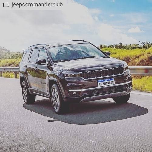
21 96437-7419 @jeepcommanderclub with 🔰 Novo Jeep Commander - O novo SUV de 7 lugares da Jeep no Brasil 🇧🇷 - Jeep Commander Limited T270 1.3 turboflex AT6 - R$ 199.990 - Jeep Commander Overland T270 1.3 turboflex AT6 R$ 219.990 - Jeep Commander Limited TD380 2.0 diesel AT9 R$ 259.990 - Jeep Commander Overland TD380 2.0 diesel AT9 R$ 279.990 Também temos descontos para cnpj ➖➖➖➖➖➖➖➖➖➖➖➖➖ #Jeep #JeepCommander #JeepLovers #JeepLover #Commander #NewCommander #NewJeepCommander #AllNewCommander #4x4 #Makehistory #OlllllllO #like4like #offroad #auto #autoshow #jeeplove #pictureoftheday #photoofday #jeepnation #car #jeepexperience #carsofinstagram #follow4follow #instacars #jeeplife #jeepcommanderclub #jeepgrandcommander #meridian #grandcommander (em Jeep | Brasil) https://www.instagram.com/p/CULHQZJFNJ4/?utm_medium=tumblr

[spiritsoulandbody]

APRIL 14, 2022 MAUNDY THURSDAY John 13 A New Commandment I Give You

https://youtu.be/oOmea43M9HE Read the full article

[max1461]

\newcommand{\shit}[1]{pissing and shitting user onrtrp into the sewers and hitting them with #1 kg frying pan}

\leq and \geq are two of my acquaintances

[iramos68]

A new commandment I give to you, that you love one another; as I have loved you, that you also love one another. By this all will know that you are My disciples, if you have love for one another.” John 13:34‭-‬35 #Agape #Love #BrotherlyLove #NewCommandment #❤️

[indirect]

https://t.co/Vp1IsClNeQ — \newcommand{\femb0t}{ (@__femb0t)

[nelcedar]

I am giving you a new commandment, that you love one another. Just as I have loved you, so you too are to love one another. John 13:34 AMP https://bible.com/bible/1588/jhn.13.34.AMP #TCInspire #tcinspire #TCI #newcommandment (at Pokuase Hills) https://www.instagram.com/p/COM2L-hh0gV/?igshid=17bpx3vrx9nho

[jameszeeshan]

Maundy Thursday A new command I give you: Love one another. As I have loved you, so you must love one another. By this everyone will know that you are my disciples, if you love one another. #HolyWeek #MaundyThursday #LastSupper #NewCommand #instaZJ #tumblrZJ #pinterestZJ #tweetZJ #linkedinZJ #quoteZJ https://www.facebook.com/570586976426543/posts/1562847983867099/?d=n&substory_index=0

[olehswift4]

\documentclass[12pt]{article}

\usepackage{pstricks}

\usepackage{pst-all}

\newcommand{\wgt}{\boldsymbol{\bar{w}}}

\usepackage{amsmath,amssymb}

\usepackage{verbatim}

\usepackage{color}

\usepackage{amsmath}

\usepackage{amssymb}

\usepackage{amsthm}

\newtheorem{theorem}{Theorem}

\newtheorem{corollary}{Corollary}[theorem]

\newtheorem{lemma}[theorem]{Lemma}

\renewcommand{\qedsymbol}{$\blacksquare$}

\DeclareMathOperator{\E}{\mathbb{E}}

\definecolor{orange}{RGB}{255,57,0}

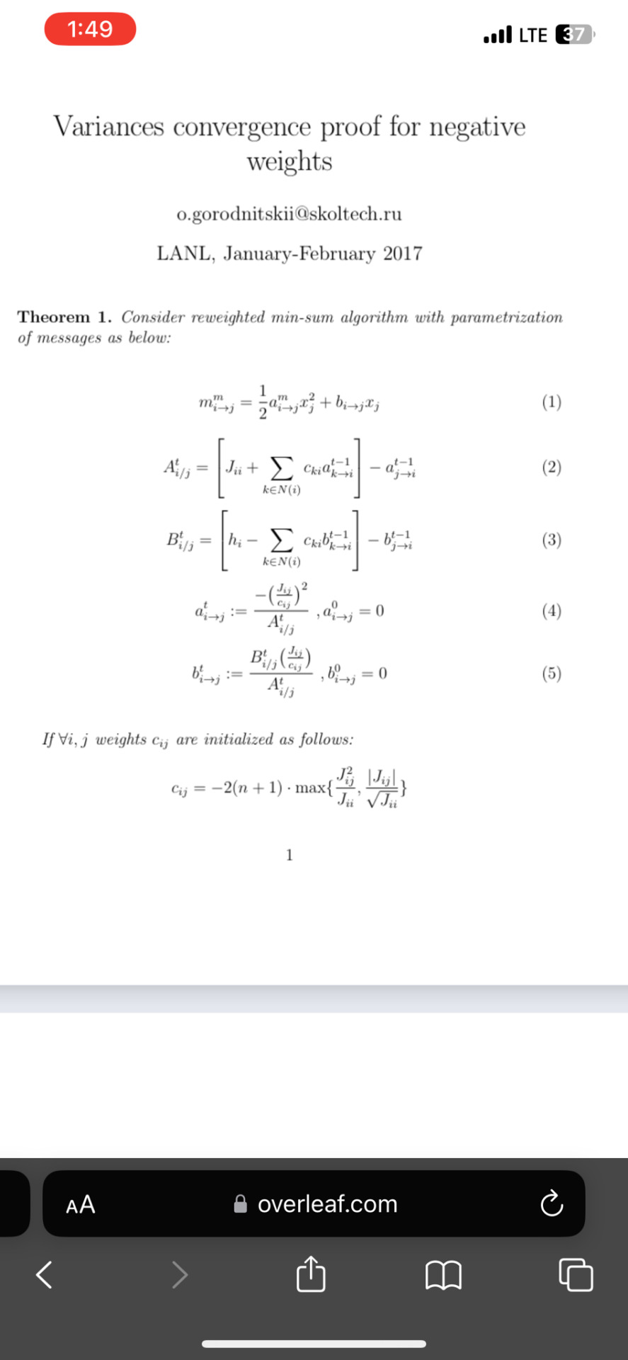
\title{Variances convergence proof for negative weights}

\author{o.gorodnitskii@skoltech.ru}

\date{LANL, January-February 2017}

\usepackage{natbib}

\usepackage{graphicx}

\begin{document}

\maketitle

\begin{theorem} Consider reweighted min-sum algorithm with parametrization of messages as below:\\

\begin{equation}

m_{i \rightarrow j}^{m} = \frac{1}{2} a_{i \rightarrow j}^{m}x_j^2 + b_{i \rightarrow j}x_j

\end{equation}

\begin{equation}

A_{i \slash j}^{t} = \left[ J_{ii} + \sum_{k \in N(i)}{c_{ki} a_{k \rightarrow i}^{t - 1}} \right] - a_{j \rightarrow i}^{t - 1}

\end{equation}

\begin{equation}

B_{i \slash j}^{t} = \left[ h_{i} - \sum_{k \in N(i)}{c_{ki} b_{k \rightarrow i}^{t - 1}} \right] - b_{j \rightarrow i}^{t - 1}

\end{equation}

\begin{equation}

a_{i \rightarrow j}^{t} := \frac{-\big( \frac{J_{ij}}{c_{ij}} \big)^2 }{A_{i \slash j}^{t}} \ , a_{i \rightarrow j}^{0} = 0

\end{equation}

\begin{equation}

b_{i \rightarrow j}^{t} := \frac{B_{i \slash j}^{t} \big( \frac{J_{ij}}{c_{ij}} \big) }{A_{i \slash j}^{t}} \ , b_{i \rightarrow j}^{0} = 0

\end{equation}\bigskip

If $\forall i,j$ weights $c_{ij}$ are initialized as follows:

$$c_{ij} = -2(n + 1) \cdot \max \{ \frac{J_{ij}^{2}}{J_{ii}}, \frac{|J_{ij}|}{\sqrt{J_{ii}}} \}$$

then sequence $a_{i \rightarrow j}^{t}$ (and variances $\text{Var}_{ij}^{t} = \frac{1}{a_{i \rightarrow j}^{t}}$) converges.\\

\end{theorem}

Proof comes below after additional lemmas.\\

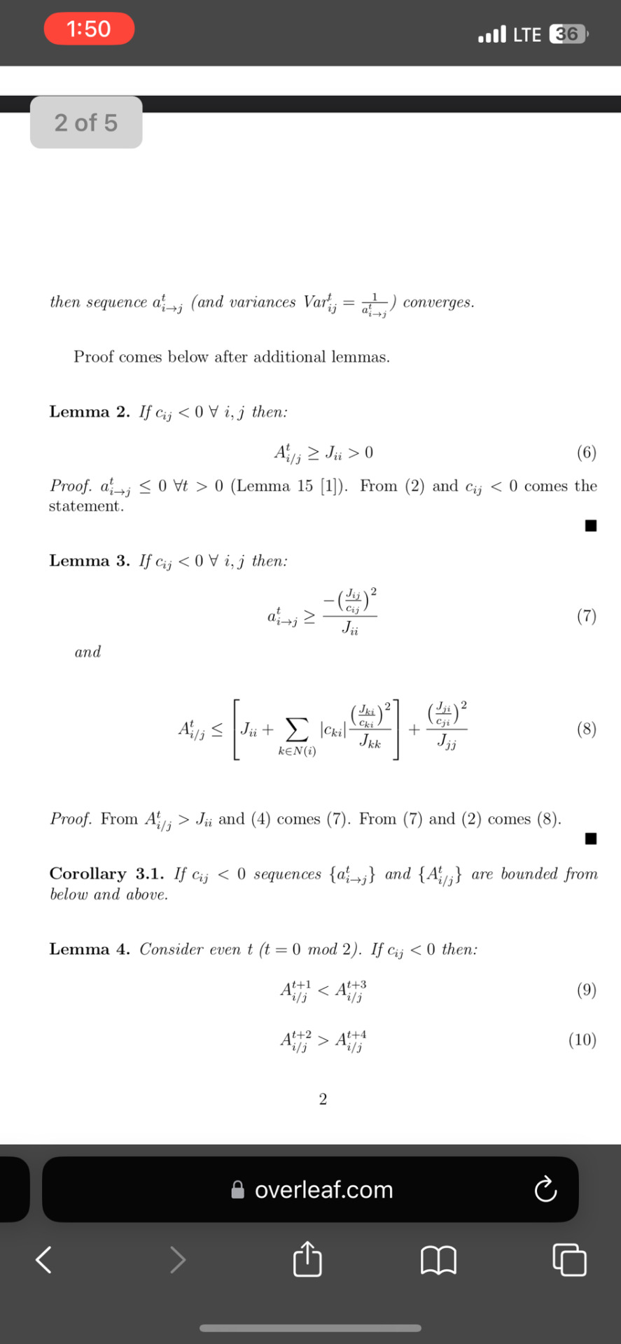
\begin{lemma} If $c_{ij} < 0 \ \forall \ i,j$ then:

\begin{equation}

A_{i \slash j}^{t} \geq J_{ii} > 0

\end{equation}

\begin{proof}

$a_{i \rightarrow j}^{t} \leq 0 \ \forall t > 0$ (Lemma 15 \cite{ruoz13}). From (2) and $c_{ij} < 0$ comes the statement.

\end{proof}

\end{lemma}

\begin{lemma}

If $c_{ij} < 0 \ \forall \ i,j$ then:

\begin{equation}

a_{i \rightarrow j}^{t} \geq \frac{-\big( \frac{J_{ij}}{c_{ij}} \big)^2}{J_{ii}}

\end{equation}

and\\

\begin{equation}

A_{i \slash j}^{t} \leq \left[ J_{ii} + \sum_{k \in N(i)}{|c_{ki}| \frac{\big( \frac{J_{ki}}{c_{ki}} \big)^2}{J_{kk}}} \right] + \frac{\big( \frac{J_{ji}}{c_{ji}} \big)^2}{J_{jj}}\\

\end{equation}\\

\begin{proof}

From $A_{i \slash j}^{t} > J_{ii}$ and (4) comes (7). From (7) and (2) comes (8).

\end{proof}

\end{lemma}

\begin{corollary}

If $c_{ij} < 0$ sequences $\{a_{i \rightarrow j}^{t}\}$ and $\{A_{i \slash j}^{t}\}$ are bounded from below and above.\\

\end{corollary}

\begin{lemma}

Consider even t ($t = 0 \ \text{mod} \ 2$). If $c_{ij} < 0$ then:

\begin{equation}

A_{i \slash j}^{t + 1} < A_{i \slash j}^{t + 3}

\end{equation}

\begin{equation}

A_{i \slash j}^{t + 2} > A_{i \slash j}^{t + 4}

\end{equation}

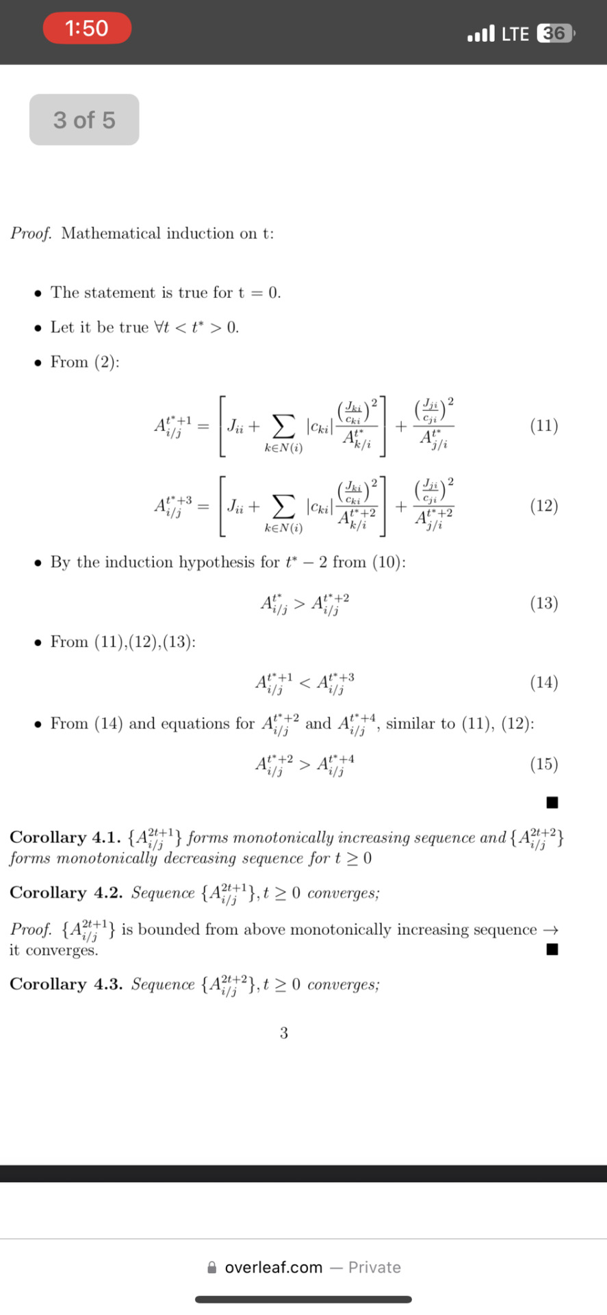
\begin{proof} Mathematical induction on t:\\

\begin{itemize}

\item The statement is true for t = 0.

\item Let it be true $\forall t < t^{*} > 0$.

\item From (2):

\begin{equation}

A_{i \slash j}^{t^{*} + 1} = \left[ J_{ii} + \sum_{k \in N(i)}{|c_{ki}| \frac{\big( \frac{J_{ki}}{c_{ki}} \big)^2}{A_{k \slash i}^{t^{*}}}} \right] + \frac{\big( \frac{J_{ji}}{c_{ji}} \big)^2}{A_{j \slash i}^{t^{*}}}

\end{equation}

\begin{equation}

A_{i \slash j}^{t^{*} + 3} = \left[ J_{ii} + \sum_{k \in N(i)}{|c_{ki}| \frac{\big( \frac{J_{ki}}{c_{ki}} \big)^2}{A_{k \slash i}^{t^{*} + 2}}} \right] + \frac{\big( \frac{J_{ji}}{c_{ji}} \big)^2}{A_{j \slash i}^{t^{*} + 2}}

\end{equation}

\item By the induction hypothesis for $t^{*} - 2$ from (10):\\

\begin{equation}

A_{i \slash j}^{t^{*}} > A_{i \slash j}^{t^{*} + 2}

\end{equation}

\item From (11),(12),(13):\\

\begin{equation}

A_{i \slash j}^{t^{*} + 1} < A_{i \slash j}^{t^{*} + 3}

\end{equation}

\item From (14) and equations for $A_{i \slash j}^{t^{*} + 2}$ and $A_{i \slash j}^{t^{*} + 4}$, similar to (11), (12):\\

\begin{equation}

A_{i \slash j}^{t^{*} + 2} > A_{i \slash j}^{t^{*} + 4}

\end{equation}

\end{itemize}

\end{proof}

\end{lemma}

\begin{corollary}

$\{A_{i \slash j}^{2t + 1}\}$ forms monotonically increasing sequence and $\{A_{i \slash j}^{2t + 2}\}$ forms monotonically decreasing sequence for $t \geq 0$

\end{corollary}

\begin{corollary}

Sequence $\{A_{i \slash j}^{2t + 1}\}, t \geq 0$ converges;

\begin{proof}

$\{A_{i \slash j}^{2t + 1}\}$ is bounded from above monotonically increasing sequence $\rightarrow$ it converges.

\end{proof}

\end{corollary}

\begin{corollary}

Sequence $\{A_{i \slash j}^{2t + 2}\}, t \geq 0$ converges;

\end{corollary}

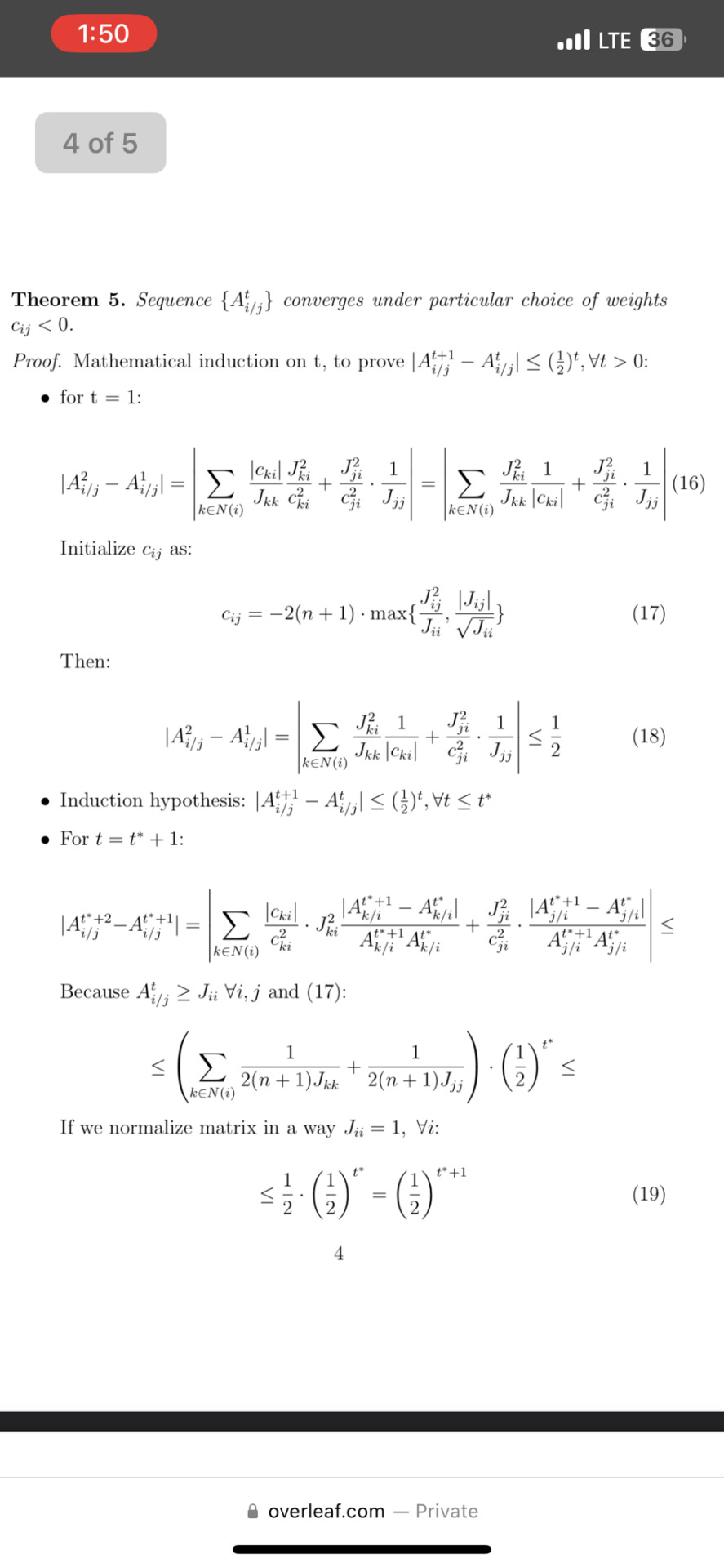
\begin{theorem}

Sequence $\{A_{i \slash j}^{t}\}$ converges under particular choice of weights $c_{ij} < 0$.

\begin{proof}

Mathematical induction on t, to prove $|A_{i \slash j}^{t + 1} - A_{i \slash j}^{t}| \leq (\frac{1}{2})^{t}, \forall t > 0$:

\begin{itemize}

\item for t = 1:

\begin{equation}

|{A_{i \slash j}^{2} - {A_{i \slash j}^{1}| = \left| \sum_{k \in N(i)}{\frac{|c_{ki}|}{J_{kk}} \frac{J_{ki}^2}{c_{ki}^2}} + \frac{J_{ji}^2}{c_{ji}^2} \cdot \frac{1}{J_{jj}} \right| = \left| \sum_{k \in N(i)}{\frac{J_{ki}^2}{J_{kk}} \frac{1}{|c_{ki}|}} + \frac{J_{ji}^2}{c_{ji}^2} \cdot \frac{1}{J_{jj}} \right|

\end{equation}

Initialize $c_{ij}$ as:

\begin{equation}

c_{ij} = -2(n + 1) \cdot \max \{ \frac{J_{ij}^{2}}{J_{ii}}, \frac{|J_{ij}|}{\sqrt{J_{ii}}} \}

\end{equation}

Then:

\begin{equation}

|A_{i \slash j}^{2} - A_{i \slash j}^{1}| = \left| \sum_{k \in N(i)}{\frac{J_{ki}^2}{J_{kk}} \frac{1}{|c_{ki}|}} + \frac{J_{ji}^2}{c_{ji}^2} \cdot \frac{1}{J_{jj}} \right| \leq \frac{1}{2}

\end{equation}

\item Induction hypothesis: $|A_{i \slash j}^{t + 1} - A_{i \slash j}^{t}| \leq (\frac{1}{2})^{t}, \forall t \leq t^{*} $

\item For $t = t^{*} + 1$:

$$|A_{i \slash j}^{t^{*} + 2} - A_{i \slash j}^{t^{*} + 1}| = \left| \sum_{k \in N(i)}{\frac{|c_{ki}|}{c_{ki}^2} \cdot {J_{ki}^2} \frac{|A_{k \slash i}^{t^{*} + 1} - A_{k \slash i}^{t^{*}}|}{A_{k \slash i}^{t^{*} + 1}A_{k \slash i}^{t^{*}}}} + \frac{J_{ji}^2}{c_{ji}^2} \cdot \frac{|A_{j \slash i}^{t^{*} + 1} - A_{j \slash i}^{t^{*}}|}{A_{j \slash i}^{t^{*} + 1}A_{j \slash i}^{t^{*}}} \right| \leq $$

Because $A_{i \slash j}^{t} \geq J_{ii} \ \forall i,j$ and (17):

$$\leq \left( \sum_{k \in N(i)}{\frac{1}{2(n + 1)J_{kk}}} + \frac{1}{2(n + 1)J_{jj}} \right) \cdot \left( \frac{1}{2} \right)^{t^{*}} \leq$$

If we normalize matrix in a way $J_{ii} = 1, \ \forall i$:

\begin{equation}

\leq \frac{1}{2} \cdot \left( \frac{1}{2} \right)^{t^{*}} = \left( \frac{1}{2} \right)^{t^{*} + 1}

\end{equation}

\end{itemize}

\end{proof}

\end{theorem}

\begin{corollary}

If $c_{ij} < 0 \ \forall i,j$ initialized according to (17), sequence $a_{i \rightarrow j}^{t}$ (and variances $\text{Var}_{ij}^{t} = \frac{1}{a_{i \rightarrow j}^{t}}$) converges.\\

\end{corollary}

\bibliographystyle{plain}

\bibliography{references}

\end{document}

[transgenderer]

as i work through a problem set i add more commands and operators to the start of my latex file to make writing certain things faster (which, btw, is the key to LaTeX), so by the end it gets...kind of out of hand

\DeclareMathOperator{\R}{\mathbb{R}}

\DeclareMathOperator{\g}{\gamma}

\DeclareMathOperator{\B}{\beta}

\DeclareMathOperator{\e}{\epsilon}

\newcommand{\pma}[1]{\begin{pmatrix}

#1

\end{pmatrix}}

\newcommand{\lr}[1]{\langle#1\rangle}

\newcommand{\pp}[2]{\frac{\partial#1}{\partial#2}}

\newcommand{\bp}[1]{\bigg(#1\bigg)}

\DeclareMathOperator{\G}{\Gamma}

\newcommand{\dd}[2]{\frac{d #1}{d #2}}

\DeclareMathOperator{\X}{\mathcal{X}}

\DeclareMathOperator{\grad}{\text{grad}}

\DeclareMathOperator{\dv}{\text{div}}

\DeclareMathOperator{\la}{\vartriangle}

\newcommand{\D}[1]{\frac{D}{d#1}}

\DeclareMathOperator{\ep}{\epsilon}

\DeclareMathOperator{\w}{\omega}

(i forgot i already defined epsilon, so when it threw a "command already defined" error i changed the name. woops)