#sub2

[lovebrewed]

☕️     ⋆     FIN!

this   feels   like   tj’s   worst   nightmare   coming   back   to   life   .   because   he   knows—   there’s   no   coming   back   from   this   .   no   amount   of   fighting   ,   no   desperate   pleas   ,   no   grand   gestures   will   change   the   way   beau   looks   at   him   now   .   the   realization   settles   deep   in   his   chest   ,   heavier   than   anything   he’s   ever   carried   .   as   much   as   he   wants   to   keep   fighting   for   them   ,   for   what   they   used   to   be   ,   he   can   see   it   so   clearly   now—   beau   is   giving   up   on   him   entirely   .   his   heart   and   mind   are   set   on   santi   ,   the   one   person   who   is   willing   to   give   beau   everything   ,   who   would   never   trade   him   for   anything   else   .

that   was   supposed   to   be   him   .

if   he   hadn’t   been   so   stupid   .   if   he   hadn’t   let   beau   go   over   a   fleeting   feeling   for   nico   .   if   he   had   only   realized   sooner   what   he   had   before   it   was   too   late   .   but   life   doesn’t   work   like   that   .   love   doesn’t   work   like   that   .   one   moment   ,   you’re   loving   someone   like   they’re   the   only   person   meant   for   you;   the   next   ,   they’re   loving   someone   else   ,   and   you’re   just   a   chapter   in   their   past   .   it’s   cruel   how   easily   people   move   on   ,   how   love   shifts   and   changes   when   you   thought   it   never   would   .   beau   moved   on   .   tj?   he   doesn’t   think   he   ever   will   .   because   if   he   could   love   nico   as   much   as   he   did   ,   then   what   he   feels   for   beau   is   bigger   than   that—   something   no   one   else   will   ever   take   the   place   of   ,   even   if   beau   no   longer   belongs   to   him   .

he   understands   beau’s   wrath   ,   his   resentment   .   that’s   why   he   chooses   to   let   go   .   he   won’t   fight   anymore   .   he   won’t   beg   .   beau   deserves   happiness   ,   peace   ,   a   love   that   isn’t   weighed   down   by   past   mistakes   .   tj   will   just   have   to   live   with   the   memories—   the   way   they   loved   each   other   when   they   were   young   and   carefree   ,   too   innocent   to   understand   what   love   really   meant   .   he’ll   keep   a   piece   of   beau   ,   even   from   a   distance   ,   even   in   the   quiet   loneliness   of   his   own   mind   .

beau’s   words   blur   in   his   ears   ,   muffled   and   distorted   ,   as   if   his   body   is   rejecting   them   .   he   doesn’t   understand   them   .   doesn’t   want   to   .   because   to   understand   means   to   accept   ,   and   he   can’t   accept   that   beau   wants   him   to   be   happy   ,   that   hoping   he   will   also   find   a   love   that   he   deserves   .   he   doesn’t   want   anyone   replacing   beau   .   period   .   if   this   is   his   punishment   ,   if   this   is   what   he   deserves   ,   then   so   be   it   .   he’ll   just   live   with   it   .   alone   .

so   ,   he   steps   back   too   .

��   i   hope   he   makes   you   happy   .   i   hope   he   gives   you   the   love   i   failed   to   give   you   .   ���   his   voice   is   steady   ,   but   his   heart   is   breaking   all   over   again   .   seeing   beau   cry   hurts   more   than   anything   .   tj   can   only   hope   this   is   the   last   time   he   has   to   see   him   like   this   .   the   last   time   he   has   to   hurt   him   .

“   i   should   go   ,   ”   he   says   quietly   ,   like   a   final   goodbye   .   “   goodbye   ,   beau   .   ”   and   with   that   ,   he   turns   away   .   walks   .   never   looks   back   .   because   if   he   does   ,   he   knows   he’ll   break   .   he’ll   beg   .   and   he’s   already   lost   him   once—   he   won’t   put   himself   through   that   again   .

  the   second   tj   steps   into   his   empty   home   ,   he   moves   like   a   man   possessed   .   he   pulls   out   his   phone   ,   makes   the   calls   he’s   been   putting   off   .   he   contacts   his   colleagues   in   the   city   ,   tells   them   he’s   accepting   the   job   offer   in   new   york   .   he   doesn’t   ask   about   the   details   .   he   just   wants   to   leave   .   as   soon   as   possible   .

that   night   ,   he   packs   everything   he   owns   ,   shoving   clothes   into   suitcases   ,   throwing   away   things   he   doesn’t   need   .   he   lists   his   place   on   airbnb   ,   a   temporary   solution   for   now   ,   but   in   truth   ,   he   knows   he’s   never   coming   back   .   by   the   time   he’s   done   ,   the   house   barely   looks   lived   in   .   no   trace   of   him   remains   .

before   he   leaves   for   good   ,   he   steps   outside   ,   pausing   in   front   of   the   garbage   bins   .   in   his   hands   ,   he   holds   a   scrapbook—   a   year’s   worth   of   memories   without   beau   .   every   single   thing   he   did   ,   every   moment   he   tried   to   capture   ,   a   way   to   remind   himself   that   life   goes   on   .   that   he   goes   on   .   at   the   back   ,   a   letter   he   wrote   for   beau   .   a   long   ,   heartfelt   message   he   was   supposed   to   give   him   for   christmas   .

it   all   feels   useless   now   .

without   hesitation   ,   he   tosses   it   into   the   bin   .   the   scrapbook   .   the   letter   .   the   remnants   of   a   life   that   no   longer   belongs   to   him   .   he   walks   away   ,   leaves   everything   and   everyone   behind   .   no   goodbyes   .   no   looking   back   .

because   if   he   does   ,   he   might   never   leave   at   all   .

[fapper]

I JUST WANT A MID SHYT TO MAKE OUT WITH AT THE FUCJING CLUBBB IS THAT TOO FAWKING MUCH TO ASK FOR OH NY GODDDDD not sub2 OLD ASS 40 YEAR OLDS GTFOOO😭😭😭😭🙏🙏🙏🙏 im on my KNEES WHERE ARE THE MEN IN THEIR MID 20S YALLL

[itsclydebitches]

SUBNAUTICA 2 TRAILER CLYDE

I KNOW I SAW!!!!!!!!! Just casually browsing my feed when that lovely alert popped up~

In all seriousness, that teaser makes me really hopeful/hyped for Sub2. I never joined the hate bandwagon for Below Zero, but I found it to just be a solid game, not one that re-captured the magic of the original. This though? This feels like og Subnautica. Even with the arrival of a friend (which might just be a nod to the promised co-op?), the whole teaser has that isolated, alienated feel to it. The world is gorgeous, but every beautiful thing posses a hidden danger. You are just a spec in the deep, dark, terrifying hole that is a foreign ocean. You're alone. The only voice for miles around is the semi-cold AI system trying to keep you alive. You're vulnerable.

There are just so many details here for a minute of info. The loud sound of your breathing. The blinking red alert light. The increasingly frantic beeping. The soft edges as your groggy brain remembers the pretty, safe surface. The fact that the crab-thing appears harmless but can still kill you with its presence alone. The "Oh shit if all the fish are swimming away there's something COMING" callback. The relief of seeing a friend show up before they're snatched by a GIANT BIO-LUMINESCENT CREATURE THAT'S JUST PERSUING ITS NATURAL INSTINCTS BUT ALSO IT'S NATURAL INSTINCTS ARE TERRIFYING." Perfect for spooky season.

(Although I'm ngl, my first thought was that Purple Dude might secretly be a friend like the Emperor Leviathan. It would fit the other parallels of that ending :D)

So yeah I'm PUMPED. Haven't been this excited for a sequel since Hades II, which admittedly hadn't been that long since EA released but STILL. I do have to decide though if I'm going to experience Sub2's EA. A part of me really wants to because a) I missed the initial EA experience and b) I'm impatient, but on the other hand the Subnautica series doesn't lend itself to incomplete play like a rogue-like does and I suspect it will be a lot more bug ridden than Hades II was when it came out... but we'll see. I'll probably join EA if only to avoid spoilers lol

[creations-of-the-dreamlight]

OMFG DO YOU THINK SUBNAUTICA THREE WILL BE US GOING BSCK TO CURE THE KARAA ON ITS SOURCE PLANET??

I still haven’t finish sub2 (ik) so maybe I’m forgetting some shit but if I remember correctly didn’t the architects bring the karaa from another planet to their home planet? And the testing to cure it was done on 4546B?

And the lore kind of solves all the loose ends for 4546b and the architects planet so where else do we have to go in this story then the very start of the Karaa? Plus I feel like a lot of people are speculating that karaa is going to be used by Alterra soooo… this is my theories but once again I am stoned and haven’t seen/done a proper play through since sub2 was pre-release.

[jams-sims]

The way I need the new character in Sub2 to be connected to the below zero. Listen give me weird ailen child from below zero. Since it seems like instead of "oh update your machine" it more "update yourself evolution 2".

Its not gonna happen but im actually super excited for subnatica 2!

[the-rookies-playbook]

I love to see a Women Win

(Amanda Nunes)

September 19, 2024 Rookie's Playbook

I’m back at it again deep diving into things I have no concept of, and today it’s the world of the UFC!  I like for my first read-through something to be an explanation of sorts so I can try and figure out exactly what is happening, and today I'm diving into the beauty of women champions. 

From my understanding there are four types of championships, there is feather-weight, bantam-weight, fly-weight, and straw-weight.  I’m not gonna lie, half of these to me sound like the same thing with AI generated names.  After doing further research it all depends on the weight of the fighter, which when I was younger used to confuse the hell out of me because I thought it was so rude to segregate people into weight categories, now however I know it’s so you don’t get absolutely murdered. 

Feather-weight(126 pounds) has no current champion, but they do have three past champions.  Amanda Nunes won in 2018 with two defenses and a TKO of 1 over her opponent Cris Cyborg.  I’m not going to sit here and lie to you either if my last name was Cyborg no one could talk to me. That is such badass.  The only knowledge I have of a TKO(Total Knockout) is when executed the fighter is left unable to complete the fight, so that is insanely hardcore to me.  Currently, the brazilian fighter has insane stats ranging from 13-2 TKO, SUB 4-2, and W-L-D 23-5-0.  Now, again I will not lie to you I only know what the TKO is.  

Sub is when a fighter ‘taps out’, yielding to their opponent so that they win.  So, that takes the badass levels down some, but hey who knows this could actually be the lowest for someone and she is the dominant woman to have ever lived.  Then the W-L-D is win, loss, or draw.  The thing that I'm getting at for Nunes is that she doesn’t believe in draws and eats up her opponent every time, 23 wins! Insane! 

Now that I know the terms let's move onto bantamweight, which is the 135 pound limit.  The current champion for this category is Raquel Pennington, with an outcome of a UD over Mayra Bueno Silva.  Now comes my next question, the hell is a UD? This is a term I have heard of and often yell out when I want to look knowledgeable, it means unanimous decision.  This is when all the judges are in agreement of which fighter is the winner, so good for Miss Pennington! 

Pennington’s stats are W-L-D 16-9-0, TKO 1-1, and sub is 1-1, not bad but not my new favorite fighter Amanda Nunes good.

Women’s flyweight is next on our list and their poundage (?) is 125.  I’m going to be honest, with all the searching and rules about the fighters weight is insane to me, what is a one pound difference in the grand scheme of it all you know? Anyway, the current champion of this category is Valentina Shevchenko who won in a unanimous decision against Alexas Grasso! Look at me knowing my terms, this is what we call development guys.   Shevchenko’s stats are W-L-D 24-4-1, TKO 8-1, and Sub 7-1.  I’m gonna be honest, Miss Nunes has my heart, but Schevchenko scares the shit outta me the most. 

The final category is straw-weight and the weight is 115 pounds, again the names just all seem too similar for my taste and I find them very much confusing but non the less I digress.  The current champion is the lady with the best cheekbones I have ever seen Zhang Weili who won against Carla Esparza with a Sub2.  Her stats rival Nunes to me with a W-L-D 25-3-0, TKO 11-1, and Sub 8-0.  She is a Chinese fighter whose career I feel I will be following closely. 

After all that research I can confirm that this is the most intriguing of the sports I have covered so far, and I simply cannot wait to learn more about it.

[penny-anna]

okay sub legacy thoughts w spoilers (by 'spoilers' i mean comments on changes made from the OG not plot spoilers) (i am a little way into the lab)

keeping the coin but moving the code to get the fuse elsewhere? DICK move. took me ages to find it. not sure if it's randomised but if it is then i think i got unlucky with the second 2 digits being 11 bcos it wasn't actually obvious that they were numbers when i found them

oughhhhh took me till sub2 to recognise the dimensional co-ordinates i was running into that's really neat and im so hype to see where we're going with that

where is the spoon and the fork... where is my classic submachine cutlery puzzle :(

i appreciate that there's more explanation for what you're doing w the chemicals in the lab (that's always been a bit of a ?? puzzle as it seems to hinge on knowledge that the player doesn't actually have so you're basically just combining items till you hit on the right combo). however i always liked the detail that you're straight up breaking in rather than hunting around for the code for entry so i wish that had been kept!!

!!!!! when re-opening the game and spotting sub 0 added to the level map

ok i need to stop now bcos it's late and also im supposed to be reducing screen time bcos of my eyes. off to bed shortly zzz good night.

[mwseo]

TWIN PEAKS

s01 - sUB

02 - sUB1 / sUB2

Fuego Camina Conmigo (1992)

03 - sUB

[locoier]

i remember like. literally two years ago talking to someone about how sub2:30 seemed almost impossible for AA and now fein has a sub2:15. that is fucking insane but also if anyone could do it it would be feinberg.

[raedas]

it is a good day bc i got a sub2 time in set yayyyyyyy

[lord-html]

#Tutorial: Switch Menu

Nesse tutorial você vai aprender a montar o Switch Menu para seu Tumblr, Blog e Afins. 

Pra quem não conhece, para aparecer o conteúdo, basta clicar no assunto desejado.

Primeiro passo -  Antes de </head> Cole isso aqui lá.

Segundo passo -  Crie os botões no seu CSS, do jeito que você quiser, vou colocar o meu, se usar, credite ok? não custa nada! 

/**Menu - Endstonight|Tumblr**/  .menutitle{color: #387377; font-family: ‘Yanone Kaffeesatz’, georgia;  font-size:16px; line-height:28px; font-weight:normal; padding:5px; margin-bottom:8px; text-align: left; letter-spacing:1px; background: #f0f0f0;text-indent : 10px;-webkit-transition-duration: .40s;} .menutitle:hover{text-indent : 19px;}

( PS: Link da Font  - <link href='http://fonts.googleapis.com/css?family=Yanone+Kaffeesatz’ rel='stylesheet’ type='text/css’>

cole antes de </head> )

Terceiro Passo -   Faça o iframe comum no seu menu, e depois monte ele, mais ou menos assim: 

<div id=“tutos” style=“display:none”>

<div class=“box”><h2>Tutoriais</h2>

<div id=“topdiv”>

<div class=“menutitle” onclick=“SwitchMenu('sub1’)” style=“cursor:pointer” >Menus</div>

<span class=“submenu” id=“sub1”>

Conteudoo

</span>  

  Obs: Se você for fazer outros menus, basta substituir o sub1 por  "sub2" , "sub3" , "sub4", você pode fazer quantos quiser. 

Obs 2: Não retire a ID “topdiv” não vai funcionais sem ela.  

[impossibletimetravelfest]

I am looking for a tutor workers Who can handle simple Typing job https://www.gn3atrk.com/2DB368NW/36M98FTS/?sub2=1.2

[eden2023]

WK4 - Testing a Potential Moderator

For the this example I used parte of the same code used um Wk3, ralatered to Salaries. It was used Salary as the moderator between years of experience and Age.

The rest of the Code:

Define income groups correctly

def Income(sal): if sal['Salary'] <= 10000:

return 1

elif sal['Salary'] <= 50000:

return 2

elif sal['Salary'] <= 100000:

return 3

elif sal['Salary'] <= 150000:

return 4

else: # This ensures salaries > 200000 are assigned group 3 return 5

data_clean['Income'] = data_clean.apply(lambda sal: Income(sal), axis=1)

Create subsets

sub1 = data_clean[data_clean['Income'] == 1] sub2 = data_clean[data_clean['Income'] == 2] sub3 = data_clean[data_clean['Income'] == 3] sub4 = data_clean[data_clean['Income'] == 4] sub5 = data_clean[data_clean['Income'] == 5]

Compute correlation for each subset separately

if len(sub1) > 1: print('Association between Age and Salary for Very Low Income Salary:') print(scipy.stats.pearsonr(sub1['Age'], sub1['Salary']))

if len(sub2) > 1: print('\nAssociation between Age and Salary for Low Income Salary:') print(scipy.stats.pearsonr(sub2['Age'], sub2['Salary']))

if len(sub3) > 1: print('\nAssociation between Age and Salary for Medium Income Salary:') print(scipy.stats.pearsonr(sub3['Age'], sub3['Salary']))

if len(sub4) > 1: print('\nAssociation between Age and Salary for High Income Salary:') print(scipy.stats.pearsonr(sub4['Age'], sub4['Salary']))

if len(sub5) > 1: print('\nAssociation between Age and Salary for Very High Income Salary:') print(scipy.stats.pearsonr(sub5['Age'], sub5['Salary']))

Bar Chart: Average Salary by Income Group

income_salary_avg = data_clean.groupby('Income')['Salary'].mean()

plt.figure(figsize=(8, 5)) sns.barplot(x=income_salary_avg.index, y=income_salary_avg.values, palette="viridis") plt.xlabel("Income Group") plt.ylabel("Average Salary") plt.title("Average Salary by Income Group") plt.xticks(ticks=range(0, 5), labels=["Very Low", "Low", "Medium", "High", "Very High"]) plt.show()

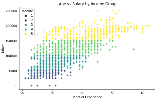
Scatter plot for Age vs Salary by Income Group

plt.figure(figsize=(8, 5)) # Set figure size sns.scatterplot( x=data_clean["Age"], y=data_clean["Salary"], hue=data_clean["Income"], # Color by Income Group palette="viridis", # Choose a color palette alpha=0.7 # Adjust transparency for better visualization ) plt.xlabel("Years of Experience") plt.ylabel("Salary") plt.title(" Age vs Salary by Income Group") plt.show()

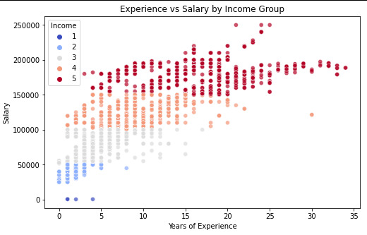
Scatter plot for Years of Experience vs Salary by Income Group

plt.figure(figsize=(8, 5)) sns.scatterplot( x=data_clean["Years of Experience"], y=data_clean["Salary"], hue=data_clean["Income"], palette="coolwarm", alpha=0.7 ) plt.xlabel("Years of Experience") plt.ylabel("Salary") plt.title("Experience vs Salary by Income Group") plt.show()

Scatter plot for Age vs Salary with Regression line styling

plt.figure(figsize=(8, 5))

sns.regplot( x=data_clean["Age"], y=data_clean["Salary"], scatter_kws={"alpha": 0.5, "color": "blue"}, # Scatter points styling line_kws={"color": "red"}, # Regression line styling ) plt.xlabel("Age") plt.ylabel("Salary") plt.title("Regression Plot: Age vs Salary") plt.show()

Scatter plot for Years of Experience vs Salary

sns.regplot( x=data_clean["Years of Experience"], y=data_clean["Salary"], scatter_kws={"alpha": 0.5, "color": "green"}, line_kws={"color": "red"}, ) plt.xlabel("Years of Experience") plt.ylabel("Salary") plt.title("Regression Plot: Years of Experience vs Salary") plt.show()

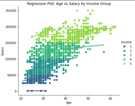
Scatter plot for Age vs Salary by Income Group

plt.figure(figsize=(8, 5))

sns.lmplot( x="Age", y="Salary", hue="Income", data=data_clean, palette="viridis", height=5, aspect=1.2 ) plt.xlabel("Age") plt.ylabel("Salary") plt.title("Regression Plot: Age vs Salary by Income Group") plt.show()

Result:

It is possible to verify that correlation between the Age and salary is for Very Low income, is -0.64, which means it ia a negative correlation and has a p-value=0.35, that is over thant p-value<0.05. so p-value for the very low it is no significante.

for the rest of the groups, Low, Medium, High and Very High, the correlation value is positive, and the p-value is unde 0.05, so we cansay that p-valeu for the rest is a significate

it is possivel to see in the Scatter plot .

[jayconner-raisingprivatemoney]

The Ultimate Guide to Buying Real Estate Using Creative Financing| William Tingle

Private Money Academy Conference:

Free Report:

William Tingle, Host of www.Sub2Deals.com is a nationally known real estate investor, investing coach, author, and public speaker. William had worked in the restaurant business for almost 20 years when in 1999, he ordered a Carleton Sheets Nothing Down course off of a late-night TV infomercial. He read it and took a $5000 advance from a credit card to start his real estate investing career.

Exactly one year later he quit his job for good, paid the credit card off, and has to this day never used a penny of his own money for investing.

For over 10 years he operated a real estate business where he wholesaled and rehabbed numerous properties each year but found his real niche in what he calls “Sub2”, buying subject to existing financing. To date, he has taken the deed on over 500 properties and even though he “retired” in Belize in 2010, he continues to buy 20 to 25 properties a year in this manner in select markets throughout the United States.

He has trained and coached countless students all over the country to become financially successful real estate investors. William has written several real estate courses. His flagship courses are “The “Ultimate” Sub2 Guidebook” & “Extreme Marketing – The “Ultimate” Marketing Guidebook”. “Ultimate Sub2” covers every aspect of “subject to” investing from marketing to finding motivated sellers, to negotiating the deal, to completing the paperwork, to how to market and sell the properties.

“Extreme Marketing” is a marketing manual with literally hundreds of both time-tested and unique, outside-the-box marketing ideas to grow your real estate business.

Timestamps:

00:01 Raising Private Without Asking For It

06:15 Struggling with Mortgage Payments

07:20 Property Sale with Retained Mortgage

11:46 Swift Real Estate Solutions Offered

16:13 Cash Buying Criteria Explained

18:24 Profitable Low-Equity House Investments

22:40 The Rise of Due on Sale Clauses

26:09 Private Lending and Second Position Strategy

27:05 Creative Financing with Seller Partnerships

30:06 Successful Real Estate Strategy

Have you read Jay’s new book: Where to Get The Money Now?

It is available FREE (all you pay is the shipping and handling) at

What is Private Money? Real Estate Investing with Jay Conner

Jay Conner is a proven real estate investment leader. He maximizes creative methods to buy and sell properties with profits averaging $67,000 per deal without using his own money or credit.

What is Real Estate Investing? Live Private Money Academy Conference

YouTube Channel

Apple Podcasts:

Facebook:

[christmascookiediary]

Would tophiachu be so hated if she wasnt sub2?

[ntaylor33]

Data Visualization - Assignment 2

For my first Python program, please see below:

-----------------------------PROGRAM--------------------------------

-- coding: utf-8 --

""" Created: 27FEB2025

@author:Nicole taylor """ import pandas import numpy

any additional libraries would be imported here

data = pandas.read_csv('GapFinder- _PDS.csv', low_memory=False)

print (len(data)) #number of observations (rows) print (len(data.columns)) # number of variables (columns)

checking the format of your variables

data['ref_area.label'].dtype

setting variables you will be working with to numeric

data['obs_value'] = pandas.to_numeric(data['obs_value'])

counts and percentages (i.e. frequency distributions) for each variable

Value1 = data['obs_value'].value_counts(sort=False) print (Value1)

PValue1 = data['obs_value'].value_counts(sort=False, normalize=True) print (PValue1)

Gender = data['sex.label'].value_counts(sort=False) print (Gender)

PGender = data['sex.label'].value_counts(sort=False, normalize=True) print (PGender)

Country = data['Country.label'].value_counts(sort=False) print (Country)

PCountry = data['Country.label'].value_counts(sort=False, normalize=True) print (PCountry)

MStatus = data['MaritalStatus.label'].value_counts(sort=False) print (MStatus)

PMStatus = data['MaritalStatus.label'].value_counts(sort=False, normalize=True) print (PMStatus)

LMarket = data['LaborMarket.label'].value_counts(sort=False) print (LMarket)

PLMarket = data['LaborMarket.label'].value_counts(sort=False, normalize=True) print (PLMarket)

Year = data['Year.label'].value_counts(sort=False) print (Year)

PYear = data['Year.label'].value_counts(sort=False, normalize=True) print (PYear)

ADDING TITLES

print ('counts for Value') Value1 = data['obs_value'].value_counts(sort=False) print (Value1)

print (len(data['TAB12MDX'])) #number of observations (rows)

print ('percentages for Value') p1 = data['obs_value'].value_counts(sort=False, normalize=True) print (PValue1)

print ('counts for Gender') Gender = data['sex.label'].value_counts(sort=False) print(Gender)

print ('percentages for Gender') p2 = data['sex.label'].value_counts(sort=False, normalize=True) print (PGender)

print ('counts for Country') Country = data['Country.label'].value_counts(sort=False, dropna=False) print(Country)

print ('percentages for Country') PCountry = data['Country.label'].value_counts(sort=False, normalize=True) print (PCountry)

print ('counts for Marital Status') MStatus = data['MaritalStatus.label'].value_counts(sort=False, dropna=False) print(MStatus)

print ('percentages for Marital Status') PMStatus = data['MaritalStatus.label'].value_counts(sort=False, dropna=False, normalize=True) print (PMStatus)

print ('counts for Labor Market') LMarket = data['LaborMarket.label'].value_counts(sort=False, dropna=False) print(LMarket)

print ('percentages for Labor Market') PLMarket = data['LaborMarket.label'].value_counts(sort=False, dropna=False, normalize=True) print (PLMarket)

print ('counts for Year') Year = data['Year.label'].value_counts(sort=False, dropna=False) print(Year)

print ('percentages for Year') PYear = data['Year.label'].value_counts(sort=False, dropna=False, normalize=True) print (PYear)

---------------------------------------------------------------------------

frequency distributions using the 'bygroup' function

print ('Frequency of Countries') TCountry = data.groupby('Country.label').size() print(TCountry)

subset data to young adults age 18 to 25 who have smoked in the past 12 months

sub1=data[(data[TCountry]='United States of America') & (data[Gender]='Sex:Female')]

make a copy of my new subsetted data

sub2 = sub1.copy()

frequency distributions on new sub2 data frame

print('counts for Country')

c5 = sub1['Country.label'].value_counts(sort=False)

print(c5)

upper-case all DataFrame column names - place afer code for loading data aboave

data.columns = list(map(str.upper, data.columns))

bug fix for display formats to avoid run time errors - put after code for loading data above

pandas.set_option('display.float_format', lambda x:'%f'%x)

-----------------------------RESULTS--------------------------------

runcell(0, 'C:/Users/oen8fh/.spyder-py3/temp.py') 85856 12 16372.131 1 7679.474 1 462.411 1 8230.246 1 4758.121 1 .. 1609.572 1 95.113 1 372.197 1 8.814 1 3.796 1 Name: obs_value, Length: 79983, dtype: int64

16372.131 0.000012 7679.474 0.000012 462.411 0.000012 8230.246 0.000012 4758.121 0.000012

1609.572 0.000012 95.113 0.000012 372.197 0.000012 8.814 0.000012 3.796 0.000012 Name: obs_value, Length: 79983, dtype: float64

Sex: Total 28595 Sex: Male 28592 Sex: Female 28595 Sex: Other 74 Name: sex.label, dtype: int64 Sex: Total 0.333058 Sex: Male 0.333023 Sex: Female 0.333058 Sex: Other 0.000862 Name: sex.label, dtype: float64 Afghanistan 210 Angola 291 Albania 696 Argentina 768 Armenia 627

Samoa 117 Yemen 36 South Africa 993 Zambia 306 Zimbabwe 261 Name: Country.label, Length: 169, dtype: int64

Afghanistan 0.002446 Angola 0.003389 Albania 0.008107 Argentina 0.008945 Armenia 0.007303

Samoa 0.001363 Yemen 0.000419 South Africa 0.011566 Zambia 0.003564 Zimbabwe 0.003040 Name: Country.label, Length: 169, dtype: float64

Marital status (Aggregate): Total 26164 Marital status (Aggregate): Single / Widowed / Divorced 26161 Marital status (Aggregate): Married / Union / Cohabiting 26156 Marital status (Aggregate): Not elsewhere classified 7375 Name: MaritalStatus.label, dtype: int64

Marital status (Aggregate): Total 0.304743 Marital status (Aggregate): Single / Widowed / Divorced 0.304708 Marital status (Aggregate): Married / Union / Cohabiting 0.304650 Marital status (Aggregate): Not elsewhere classified 0.085900 Name: MaritalStatus.label, dtype: float64

Labour market status: Total 21870 Labour market status: Employed 21540 Labour market status: Unemployed 20736 Labour market status: Outside the labour force 21710 Name: LaborMarket.label, dtype: int64

Labour market status: Total 0.254729 Labour market status: Employed 0.250885 Labour market status: Unemployed 0.241521 Labour market status: Outside the labour force 0.252865 Name: LaborMarket.label, dtype: float64

2021 3186 2020 3641 2017 4125 2014 4014 2012 3654 2022 3311 2019 4552 2011 3522 2009 3054 2004 2085 2023 2424 2018 3872 2016 3843 2015 3654 2013 3531 2010 3416 2008 2688 2007 2613 2005 2673 2002 1935 2006 2700 2024 372 2003 2064 2001 1943 2000 1887 1999 1416 1998 1224 1997 1086 1996 999 1995 810 1994 714 1993 543 1992 537 1991 594 1990 498 1989 462 1988 423 1987 423 1986 357 1985 315 1984 273 1983 309 1982 36 1980 36 1970 42 Name: Year.label, dtype: int64

2021 0.037109 2020 0.042408 2017 0.048046 2014 0.046753 2012 0.042560 2022 0.038565 2019 0.053019 2011 0.041022 2009 0.035571 2004 0.024285 2023 0.028233 2018 0.045099 2016 0.044761 2015 0.042560 2013 0.041127 2010 0.039788 2008 0.031308 2007 0.030435 2005 0.031134 2002 0.022538 2006 0.031448 2024 0.004333 2003 0.024040 2001 0.022631 2000 0.021979 1999 0.016493 1998 0.014256 1997 0.012649 1996 0.011636 1995 0.009434 1994 0.008316 1993 0.006325 1992 0.006255 1991 0.006919 1990 0.005800 1989 0.005381 1988 0.004927 1987 0.004927 1986 0.004158 1985 0.003669 1984 0.003180 1983 0.003599 1982 0.000419 1980 0.000419 1970 0.000489 Name: Year.label, dtype: float64

counts for Value 16372.131 1 7679.474 1 462.411 1 8230.246 1 4758.121 1 .. 1609.572 1 95.113 1 372.197 1 8.814 1 3.796 1 Name: obs_value, Length: 79983, dtype: int64

percentages for Value 16372.131 0.000012 7679.474 0.000012 462.411 0.000012 8230.246 0.000012 4758.121 0.000012

1609.572 0.000012 95.113 0.000012 372.197 0.000012 8.814 0.000012 3.796 0.000012 Name: obs_value, Length: 79983, dtype: float64

counts for Gender Sex: Total 28595 Sex: Male 28592 Sex: Female 28595 Sex: Other 74 Name: sex.label, dtype: int64

percentages for Gender Sex: Total 0.333058 Sex: Male 0.333023 Sex: Female 0.333058 Sex: Other 0.000862 Name: sex.label, dtype: float64

counts for Country Afghanistan 210 Angola 291 Albania 696 Argentina 768 Armenia 627

Samoa 117 Yemen 36 South Africa 993 Zambia 306 Zimbabwe 261 Name: Country.label, Length: 169, dtype: int64

percentages for Country Afghanistan 0.002446 Angola 0.003389 Albania 0.008107 Argentina 0.008945 Armenia 0.007303

Samoa 0.001363 Yemen 0.000419 South Africa 0.011566 Zambia 0.003564 Zimbabwe 0.003040 Name: Country.label, Length: 169, dtype: float64

counts for Marital Status Marital status (Aggregate): Total 26164 Marital status (Aggregate): Single / Widowed / Divorced 26161 Marital status (Aggregate): Married / Union / Cohabiting 26156 Marital status (Aggregate): Not elsewhere classified 7375 Name: MaritalStatus.label, dtype: int64

percentages for Marital Status Marital status (Aggregate): Total 0.304743 Marital status (Aggregate): Single / Widowed / Divorced 0.304708 Marital status (Aggregate): Married / Union / Cohabiting 0.304650 Marital status (Aggregate): Not elsewhere classified 0.085900 Name: MaritalStatus.label, dtype: float64

counts for Labor Market Labour market status: Total 21870 Labour market status: Employed 21540 Labour market status: Unemployed 20736 Labour market status: Outside the labour force 21710 Name: LaborMarket.label, dtype: int64

percentages for Labor Market Labour market status: Total 0.254729 Labour market status: Employed 0.250885 Labour market status: Unemployed 0.241521 Labour market status: Outside the labour force 0.252865 Name: LaborMarket.label, dtype: float64

counts for Year 2021 3186 2020 3641 2017 4125 2014 4014 2012 3654 2022 3311 2019 4552 2011 3522 2009 3054 2004 2085 2023 2424 2018 3872 2016 3843 2015 3654 2013 3531 2010 3416 2008 2688 2007 2613 2005 2673 2002 1935 2006 2700 2024 372 2003 2064 2001 1943 2000 1887 1999 1416 1998 1224 1997 1086 1996 999 1995 810 1994 714 1993 543 1992 537 1991 594 1990 498 1989 462 1988 423 1987 423 1986 357 1985 315 1984 273 1983 309 1982 36 1980 36 1970 42 Name: Year.label, dtype: int64

percentages for Year 2021 0.037109 2020 0.042408 2017 0.048046 2014 0.046753 2012 0.042560 2022 0.038565 2019 0.053019 2011 0.041022 2009 0.035571 2004 0.024285 2023 0.028233 2018 0.045099 2016 0.044761 2015 0.042560 2013 0.041127 2010 0.039788 2008 0.031308 2007 0.030435 2005 0.031134 2002 0.022538 2006 0.031448 2024 0.004333 2003 0.024040 2001 0.022631 2000 0.021979 1999 0.016493 1998 0.014256 1997 0.012649 1996 0.011636 1995 0.009434 1994 0.008316 1993 0.006325 1992 0.006255 1991 0.006919 1990 0.005800 1989 0.005381 1988 0.004927 1987 0.004927 1986 0.004158 1985 0.003669 1984 0.003180 1983 0.003599 1982 0.000419 1980 0.000419 1970 0.000489 Name: Year.label, dtype: float64

Frequency of Countries Country.label Afghanistan 210 Albania 696 Angola 291 Antigua and Barbuda 87 Argentina 768

Viet Nam 639 Wallis and Futuna 117 Yemen 36 Zambia 306 Zimbabwe 261 Length: 169, dtype: int64

-----------------------------REVIEW--------------------------------

So as you can see in the results. I was able to show the Year, Marital Status, Labor Market, and the Country. I'm still a little hazy on the sub1, but overall it was a good basic start.