#regression analysis Multiple Regression Data Analysis

[romanticize-until-you-drop]

So I just won a competition for my research project…

MOM DAD IM A REAL SCIENTIST!!

[darkmaga-retard]

Despite the endless barrage of propaganda by the mainstream media and global elites, it turns out that man-made fossil fuel emissions have “zero impact” on climate change.

A groundbreaking new study challenges the belief that human emissions are the primary driver of increasing atmospheric carbon dioxide (CO2) concentrations. The research, published in the Science of Climate Change, concludes that sea surface temperatures (SST) play a far more significant role than anthropogenic (human-caused) factors in determining annual changes in atmospheric CO2 levels.

Naturalnews.com reports: Using multivariate analysis and publicly available data from leading climate and energy organizations, Dao Ato’s study compares the impacts of sea surface temperature and human emissions on atmospheric CO2 concentrations. The analysis spanned from 1959 to 2022 and employed multiple linear regression techniques to evaluate the influence of sea surface temperature and human CO? emissions on the annual increase in atmospheric CO2.

The results reveal that sea surface temperature data, derived from NASA and the UK-HADLEY Centre datasets, was the most accurate predictor of CO2 concentrations. The regression model incorporating sea surface temperature explained approximately 66% of the variance in annual CO2 increases post-1959, with a remarkably high correlation between predicted and actual CO2 levels. The study found a Pearson correlation coefficient of 0.9995 between the CO2 concentrations predicted using sea surface temperature data from the UK-HADLEY Centre and actual measurements from NOAA, with a minimal prediction error of 1.45 ppm in 2022. In contrast, human CO2 emissions showed no significant correlation with annual changes in atmospheric CO2.

Ato’s study also found that human methane emissions, despite rising dramatically in recent decades, have not contributed to rising methane concentrations in the atmosphere through the 21st century.

[covid-safer-hotties]

Long COVID symptom severity varies widely by age, gender, and socioeconomic status - Published Sept 2, 2024

By Dr. Sushama R. Chaphalkar, PhD.

In a recent study published in the journal JRSM Open, researchers analyze self-reported symptoms of long coronavirus disease 2019 (LC) from individuals using a healthcare app to examine the potential impact of demographic factors on the severity of symptoms. The researchers found that LC symptom severity varied significantly by age, gender, race, education, and socioeconomic status.

Research highlights the urgent need for targeted interventions as age, gender, and social factors play a crucial role in the intensity of long COVID symptoms. What factors increase the risk of long COVID? Several months after recovering from coronavirus disease 2019 (COVID-19), patients with LC may continue to suffer from numerous symptoms, some of which include fatigue, brain fog, and chest pain. The prevalence of LC varies, with estimates ranging from 10-30% in non-hospitalized cases to 50-70% in hospitalized patients.

Although several digital health interventions (DHIs) and applications have been developed to monitor acute symptoms of COVID-19, few have been designed to track long-term symptoms of the disease. One DHI called "Living With COVID Recovery" (LWCR) was initiated to help individuals manage LC by self-reporting symptoms and tracking their intensity. However, there remains a lack of evidence on the risk factors, characteristics, and predictors of LC, thereby limiting the accurate identification of high-risk patients to target preventive strategies.

About the study In the present study, researchers investigate the prevalence and intensity of self-reported LC symptoms to analyze their potential relationship with demographic factors to inform targeted interventions and management strategies. To this end, LWCR was used to monitor and analyze self-reported LC symptoms from individuals in 31 LC clinics throughout England and Wales.

The study included 1,008 participants who reported 1,604 unique symptoms. All patients provided informed consent for the use of their anonymized data for research.

Multiple linear regression analysis was used to explore the relationship between symptom intensity and factors such as time since registration, age, ethnicity, education, gender, and socioeconomic status through indices of multiple deprivation (IMD) on a scale of one to 10.

Education was classified into four levels denoted as NVQ 1-2, NVQ 3, NVQ 4, and NVQ 5, which reflected those who were least educated at A level, degree level, and postgraduate level, respectively. The intensity of symptoms was measured on a scale from zero to 10, with zero being the lowest and 10 the highest intensity. Descriptive statistics identified variations in symptom intensity across different demographic groups.

Study findings Although 23% of patients experienced symptoms only once, 77% experienced symptoms multiple times. Corroborating with existing literature, the most prevalent symptoms included pain, neuropsychological issues, fatigue, and dyspnea, which affected 26.5%, 18.4%, 14.3%, and 7.4% of the cohort, respectively. Symptoms such as palpitations, light-headedness, insomnia, cough, diarrhea, and tinnitus were less prevalent.

Fifteen most prevalent LC symptoms. Multiple linear regression analysis revealed that symptom intensity was significantly associated with age, gender, ethnicity, education, and IMD decile. More specifically, individuals 68 years of age and older reported higher symptom intensity by 32.5% and 86%, respectively. These findings align with existing literature that highlights the increased risk of LC symptoms with age, which may be due to weakened immunity or the presence of comorbidities. Thus, they emphasize the need for targeted interventions for this population.

Females also reported higher symptom intensity than males, by 9.2%. Non-White individuals experienced higher symptom intensity by 23.5% as compared to White individuals.

Individuals with higher education levels reported up to 47% reduced symptom intensity as compared to those with lower education levels. Higher IMD deciles, which reflect less deprived areas, were associated with lower symptom intensity; however, no significant association was observed between the number of symptoms reported and the IMD decile.

Regression results with 95% confidence interval. Note: For age, the base group is people in the age category 18–27. For IMD, the base group is people from IMD decile 1. For education, the base group is people who left school before A-level (NVQ 1–2). A significant positive association was observed between symptom intensity and the duration between registration on the app and initial symptom reporting. This finding suggests individuals may become more aware of their symptoms or that worsening symptoms prompt reporting.

Some limitations of the current study include the lack of data on comorbidities, hospitalization, and vaccine status. There is also a potential for bias against individuals lacking technological proficiency or access, which may affect the sample's representativeness, particularly for older, socioeconomically disadvantaged, or non-English-speaking individuals. Excluding patients with severe symptoms or those who were ineligible for the app may also skew the findings.

Conclusions There remains an urgent need to develop targeted interventions to address the severity of LC in relation to age, ethnicity, and socioeconomic factors. LC treatment should prioritize prevalent symptoms like pain, neuropsychological issues, fatigue, and dyspnea while also considering other possible symptoms. Furthermore, sustained support for LC clinics is essential to effectively manage the wide range of symptoms and complexities associated with LC and improve public health outcomes in the post-pandemic era.

Journal reference:

Sunkersing, D., Goodfellow, H., Mu, Y., et al. (2024). Long COVID symptoms and demographic associations: A retrospective case series study using healthcare application data. JRSM Open 15(7). doi:10.1177/20542704241274292.

journals.sagepub.com/doi/10.1177/20542704241274292

[anarchywoofwoof]

so today, a new study was released by the Institute on Taxation & Economic Policy and it's all about how the richest 1% in 41 states are literally paying less in taxes than the rest of us.

you heard that right. while the average person is out here struggling to make ends meet, the data reveals a truth that you probably already suspected: the ultra-wealthy are basically getting a free pass.

this isn't just some random report. it's a detailed analysis of tax systems across all 50 states and DC, looking at how different income groups are taxed. and the findings are kind of infuriating.

first off, most state and local tax systems are regressive in nature. this means they hit the low- and middle-income families the hardest. the bottom 20% are paying tax rates almost 60% higher than the top 1%.

and here's the kicker – in 41 out of 50 states, the rich are taxed at lower rates than everyone else. we're talking about the top 1% of earners here. they're literally paying less than any other income group.

if we look solely at Appendix A and Appendix B from the data, for example:

Appendix A - Tax Burden by Income Group: this tab on the worksheet shows the total state and local taxes as a share of family income for different income groups in each state. the columns represent different income groups, ranging from the lowest 20% of income earners in the given state to the top 1%. you can get the per capita income by state here.

for instance, in Alabama, the lowest 20% of earners pay about 11.87% of their income in taxes, while the top 1% pay only about 5.38%.

likewise, in Alaska, the lowest 20% pay around 8.71%, and the top 1% pay about 2.78%.

Appendix B - Tax Inequality Index: this section ranks states based on their tax inequality index and provides effective tax rates for different groups. states like Florida and Washington rank highest in terms of tax regressivity.

for example, in Florida, the lowest 20% pay an effective tax rate of 13.17%, while the top 1% pay just 2.74%.

Washington shows a similar pattern with the lowest 20% paying 13.80% and the top 1% paying 4.05%.

oh, and if you're low-income, it's even worse. in 34 states, low-income families are taxed at higher rates than anyone else. these are people who can barely afford to pay their bills, and they're being taxed higher than the richest people in the state.

the most regressive tax systems are in Florida, Washington, Tennessee, Nevada, South Dakota, Texas, Arkansas, and Louisiana. these places lean heavily on sales and excise taxes, which hit the poorest the hardest. states that are often branded as "low tax" – like Florida and Texas – are actually high-tax hells for low-income families.

some states are actually trying to fix this mess. New Mexico, Massachusetts, and even Washington are making moves toward less regressive taxes. they're making efforts to up taxes on the rich and giving some relief to the rest of us.

on the flip side however, some states are just making things worse. Arizona, Kentucky, South Dakota, and others are cutting taxes for the wealthy and screwing over low-income families even more. between 2021 and 2023, twenty-six states in total cut their personal income tax rates and/or corporate income tax rates, 13 of them multiple times

this report should serve as a wake-up call. it's showing us in black and white math how rigged the system is against the average person. the bottom line is that the rich are getting richer, and they're doing it at the expense of the rest of us. it's time to start calling out the gross disparity a little louder for the people in the back.

[religion-is-a-mental-illness]

Abstract

Objective: To assess the association between transgender or gender-questioning identity and screen use (recreational screen time and problematic screen use) in a demographically diverse national sample of early adolescents in the U.S.

Methods: We analyzed cross-sectional data from Year 3 of the Adolescent Brain Cognitive DevelopmentSM Study (ABCD Study®, N = 9859, 2019-2021, mostly 12-13-years-old). Multiple linear regression analyses estimated the associations between transgender or questioning gender identity and screen time, as well as problematic use of video games, social media, and mobile phones, adjusting for confounders.

Results: In a sample of 9859 adolescents (48.8% female, 47.6% racial/ethnic minority, 1.0% transgender, 1.1% gender-questioning), transgender adolescents reported 4.51 (95% CI 1.17-7.85) more hours of total daily recreational screen time including more time on television/movies, video games, texting, social media, and the internet, compared to cisgender adolescents. Gender-questioning adolescents reported 3.41 (95% CI 1.16-5.67) more hours of total daily recreational screen time compared to cisgender adolescents. Transgender identification and questioning one's gender identity was associated with higher problematic social media, video game, and mobile phone use, compared to cisgender identification.

Conclusions: Transgender and gender-questioning adolescents spend a disproportionate amount of time engaging in screen-based activities and have more problematic use across social media, video game, and mobile phone platforms.

Introduction

Screen-based digital media is integral to the daily lives of adolescents in multifaceted ways [1] but problematic screen use (characterized by inability to control usage and detrimental consequences from excessive use including preoccupation, tolerance, relapse, withdrawal, and conflict) [2], [3], has been linked with harmful mental and physical health outcomes, such as depression, poor sleep, and cardiometabolic disease [4], [5]. Transgender and gender-questioning adolescents (i.e., adolescents who are questioning their gender identity) experience a higher prevalence of bullying (adjusted prevalence ratio [aPR] 1.88 and 1.62), suicide attempts (aPR 2.65 and 2.26), and binge drinking (aPR 1.80 and 1.50), respectively, compared to their cisgender peers [6], [7], [8], [9], [10]. Transgender and gender-questioning adolescents may engage in screen-based activities that are problematic and associated with negative health outcomes but also in a way that is different from their cisgender peers in order to form communities, explore health education about their gender identity, and seek refuge from isolating or unsafe environments [11].

One study found that sexual and gender minority (SGM) adolescents (e.g., lesbian, gay, bisexual, and transgender), aged 13–18 years old, spent an average of 5 h per day online, approximately 45 min more than non-SGM adolescents in 2010–2011 [12]. However, this study grouped SGM together as a single group, conflating the experiences of gender minorities (e.g., transgender, gender-questioning) with those of sexual minorites (e.g., lesbian, gay, bisexual), and the data are now over a decade old. In a nationally representative sample of adolescents aged 13–18 years old in the U.S., transgender adolescents had higher probabilities of problematic internet use than cisgender adolescents. However, this analysis did not measure modality-specific problematic screen use such as problematic social media, video game, or mobile phone use, which may further inform the function that media use plays in the lives of gender minority adolescents [13]. While this prior research provides important groundwork to understand screen time and problematic use in gender minority adolescents, gaps remain in understanding differences in screen time and specific modalities of problematic screen use in gender minority early adolescents.

Our study aims to address the gaps in the current literature by studying associations between transgender and gender-questioning identity and screen time across several modalities including recreational and problematic social media, video game, and mobile phone use in a large, national sample of early adolescents. We hypothesized that among early adolescents, transgender identification and questioning one’s gender identity would be positively associated with greater recreational screen time and problematic screen use compared to cisgender identification.

==

tl;dr: Gender-mania is an online social contagion.

No shit. That's why these "authentic selves" and "innate identities" tend to evaporate when kids are detoxed from the internet.

[tech-insides]

What are the skills needed for a data scientist job?

It’s one of those careers that’s been getting a lot of buzz lately, and for good reason. But what exactly do you need to become a data scientist? Let’s break it down.

Technical Skills

First off, let's talk about the technical skills. These are the nuts and bolts of what you'll be doing every day.

Programming Skills: At the top of the list is programming. You’ll need to be proficient in languages like Python and R. These are the go-to tools for data manipulation, analysis, and visualization. If you’re comfortable writing scripts and solving problems with code, you’re on the right track.

Statistical Knowledge: Next up, you’ve got to have a solid grasp of statistics. This isn’t just about knowing the theory; it’s about applying statistical techniques to real-world data. You’ll need to understand concepts like regression, hypothesis testing, and probability.

Machine Learning: Machine learning is another biggie. You should know how to build and deploy machine learning models. This includes everything from simple linear regressions to complex neural networks. Familiarity with libraries like scikit-learn, TensorFlow, and PyTorch will be a huge plus.

Data Wrangling: Data isn’t always clean and tidy when you get it. Often, it’s messy and requires a lot of preprocessing. Skills in data wrangling, which means cleaning and organizing data, are essential. Tools like Pandas in Python can help a lot here.

Data Visualization: Being able to visualize data is key. It’s not enough to just analyze data; you need to present it in a way that makes sense to others. Tools like Matplotlib, Seaborn, and Tableau can help you create clear and compelling visuals.

Analytical Skills

Now, let’s talk about the analytical skills. These are just as important as the technical skills, if not more so.

Problem-Solving: At its core, data science is about solving problems. You need to be curious and have a knack for figuring out why something isn’t working and how to fix it. This means thinking critically and logically.

Domain Knowledge: Understanding the industry you’re working in is crucial. Whether it’s healthcare, finance, marketing, or any other field, knowing the specifics of the industry will help you make better decisions and provide more valuable insights.

Communication Skills: You might be working with complex data, but if you can’t explain your findings to others, it’s all for nothing. Being able to communicate clearly and effectively with both technical and non-technical stakeholders is a must.

Soft Skills

Don’t underestimate the importance of soft skills. These might not be as obvious, but they’re just as critical.

Collaboration: Data scientists often work in teams, so being able to collaborate with others is essential. This means being open to feedback, sharing your ideas, and working well with colleagues from different backgrounds.

Time Management: You’ll likely be juggling multiple projects at once, so good time management skills are crucial. Knowing how to prioritize tasks and manage your time effectively can make a big difference.

Adaptability: The field of data science is always evolving. New tools, techniques, and technologies are constantly emerging. Being adaptable and willing to learn new things is key to staying current and relevant in the field.

Conclusion

So, there you have it. Becoming a data scientist requires a mix of technical prowess, analytical thinking, and soft skills. It’s a challenging but incredibly rewarding career path. If you’re passionate about data and love solving problems, it might just be the perfect fit for you.

Good luck to all of you aspiring data scientists out there!

[fixomnia-scribble]

I think - I think - I just cracked the last big issue in my stats data analysis for my presentation. If I'm right, my remaining workload just went way down and I will be able to get around to actual presentation prep very soon.

For those who speak Stats, I'm at the stage of cross-checking the validity of my two extracted Principal Components by way of multiple linear regression against other related variables. Why? Because we're not allowed to use the much faster Cronbach's Alpha tool. We're supposed to show we understand how our models work, not just report output numbers. That's easy enough, but my dataset stinks for this particular type of analysis (My beloved prof called it "hilariously awful"), and I have had to create some pretty wild dummy variables to test against.

If this sounds like gibberish, you're not wrong.

Have planned an Indian dinner and mindless movie night with friend, after presentation.

[mvishnukumar]

Can statistics and data science methods make predicting a football game easier?

Hi,

Statistics and data science methods can significantly enhance the ability to predict the outcomes of football games, though they cannot guarantee results due to the inherent unpredictability of sports. Here’s how these methods contribute to improving predictions:

Data Collection and Analysis: 

Collecting and analyzing historical data on football games provides a basis for understanding patterns and trends. This data can include player statistics, team performance metrics, match outcomes, and more. Analyzing this data helps identify factors that influence game results and informs predictive models.

Feature Engineering:

 Feature engineering involves creating and selecting relevant features (variables) that contribute to the prediction of game outcomes. For football, features might include team statistics (e.g., goals scored, possession percentage), player metrics (e.g., player fitness, goals scored), and contextual factors (e.g., home/away games, weather conditions). Effective feature engineering enhances the model’s ability to capture important aspects of the game.

Predictive Modeling: 

Various predictive models can be used to forecast football game outcomes. Common models include:

Logistic Regression: This model estimates the probability of a binary outcome (e.g., win or lose) based on input features.

Random Forest: An ensemble method that builds multiple decision trees and aggregates their predictions. It can handle complex interactions between features and improve accuracy.

Support Vector Machines (SVM): A classification model that finds the optimal hyperplane to separate different classes (e.g., win or lose).

Poisson Regression: Specifically used for predicting the number of goals scored by teams, based on historical goal data.

Machine Learning Algorithms: 

Advanced machine learning algorithms, such as gradient boosting and neural networks, can be employed to enhance predictive accuracy. These algorithms can learn from complex patterns in the data and improve predictions over time.

Simulation and Monte Carlo Methods: 

Simulation techniques and Monte Carlo methods can be used to model the randomness and uncertainty inherent in football games. By simulating many possible outcomes based on historical data and statistical models, predictions can be made with an understanding of the variability in results.

Model Evaluation and Validation: 

Evaluating the performance of predictive models is crucial. Metrics such as accuracy, precision, recall, and F1 score can assess the model’s effectiveness. Cross-validation techniques ensure that the model generalizes well to new, unseen data and avoids overfitting.

Consideration of Uncertainty: 

Football games are influenced by numerous unpredictable factors, such as injuries, referee decisions, and player form. While statistical models can account for many variables, they cannot fully capture the uncertainty and randomness of the game.

Continuous Improvement: 

Predictive models can be continuously improved by incorporating new data, refining features, and adjusting algorithms. Regular updates and iterative improvements help maintain model relevance and accuracy.

In summary, statistics and data science methods can enhance the ability to predict football game outcomes by leveraging historical data, creating relevant features, applying predictive modeling techniques, and continuously refining models. While these methods improve the accuracy of predictions, they cannot eliminate the inherent unpredictability of sports. Combining statistical insights with domain knowledge and expert analysis provides the best approach for making informed predictions.

[thara333]

Selenium: Revolutionizing Web Testing in the Digital Age

In the rapidly advancing world of software development, ensuring the reliability and quality of web applications is paramount. Selenium, an open-source framework, has emerged as a game-changer in the realm of automated web testing. Embracing Selenium's capabilities becomes even more accessible and impactful with Selenium Training in Bangalore. This training equips individuals with the skills and knowledge to harness the full potential of Selenium, enabling them to proficiently navigate web automation challenges and contribute effectively to their respective fields. This comprehensive blog explores the multifaceted advantages of Selenium, shedding light on why it has become the go-to choice for quality assurance professionals and developers alike.

The Pinnacle of Cross-Browser Compatibility

A noteworthy strength of Selenium lies in its ability to seamlessly support multiple web browsers. Whether it's Chrome, Firefox, Edge, or others, Selenium ensures that web automation scripts deliver consistent and reliable performance across diverse platforms. This cross-browser compatibility is a crucial factor in the ever-expanding landscape of browser choices.

Programming Language Agnosticism: Bridging Accessibility Gaps

Selenium takes accessibility to the next level by being language-agnostic. Developers can write automation scripts in their preferred programming language, be it Java, Python, C#, Ruby, or others. This flexibility not only caters to diverse skill sets but also fosters collaboration within cross-functional teams, breaking down language barriers.

Seamless Interaction with Web Elements: Precision in Testing

Testing the functionality of web applications requires precise interaction with various elements such as buttons, text fields, and dropdowns. Selenium facilitates this with ease, providing testers the tools needed for comprehensive and meticulous web application testing. The ability to simulate user interactions is a key feature that sets Selenium apart.

Automated Testing: Unleashing Efficiency and Accuracy

Quality assurance professionals leverage Selenium for automated testing, a practice that not only enhances efficiency but also ensures accuracy in identifying issues and regressions throughout the development lifecycle. The power of Selenium in automating repetitive testing tasks allows teams to focus on more strategic aspects of quality assurance.

Web Scraping Capabilities: Extracting Insights from the Web

Beyond testing, Selenium is a preferred choice for web scraping tasks. Its robust features enable the extraction of valuable data from websites, opening avenues for data analysis or integration into other applications. This dual functionality enhances the versatility of Selenium in addressing various needs within the digital landscape.

Integration with Testing Frameworks: Collaborative Development Efforts

Selenium seamlessly integrates with various testing frameworks and continuous integration (CI) tools, turning it into an integral part of the software development lifecycle. This integration not only streamlines testing processes but also promotes collaboration among developers, testers, and other stakeholders, ensuring a holistic approach to quality assurance.

Thriving on Community Support: A Collaborative Ecosystem

Backed by a vast and active user community, Selenium thrives on collaboration. Continuous updates, extensive support, and a wealth of online resources create a dynamic ecosystem for learning and troubleshooting. The community-driven nature of Selenium ensures that it stays relevant and evolves with the ever-changing landscape of web technologies.

Open-Source Nature: Fostering Innovation and Inclusivity

As an open-source tool, Selenium fosters innovation and inclusivity within the software testing community. It eliminates financial barriers, allowing organizations of all sizes to benefit from its features. The collaborative spirit of open source has propelled Selenium to the forefront of web testing tools.

Parallel Test Execution: Optimizing Testing Cycles

For large-scale projects, Selenium's support for parallel test execution is a game-changer. This feature ensures faster testing cycles and efficient utilization of resources. As the demand for rapid software delivery grows, the ability to run tests concurrently becomes a crucial factor in maintaining agility.

A Robust Ecosystem Beyond the Basics

Selenium offers a robust ecosystem that goes beyond the fundamental features. Tools like Selenium Grid for parallel test execution and Selenium WebDriver for browser automation enhance its overall capabilities. This ecosystem provides users with the flexibility to adapt Selenium to their specific testing requirements.

Dynamic Waits and Synchronization: Adapting to the Dynamic Web

The dynamic nature of web applications requires a testing framework that can adapt. Selenium addresses this challenge with dynamic waits and synchronization mechanisms. These features ensure that scripts can handle delays effectively, providing reliability in testing even in the face of a rapidly changing web environment.

Continuous Updates and Enhancements: Staying Ahead of the Curve

In the fast-paced world of web technologies, staying updated is crucial. Selenium's active maintenance ensures regular updates and enhancements. This commitment to evolution allows Selenium to remain compatible with the latest browsers and technologies, positioning it at the forefront of web testing innovation.

Selenium stands as a testament to the evolution of web testing methodologies. From its cross-browser compatibility to continuous updates and a thriving community, Selenium embodies the qualities essential for success in the dynamic digital landscape. Embrace Selenium, and witness a transformative shift in your approach to web testing—where efficiency, accuracy, and collaboration converge to redefine the standards of quality assurance in the digital age. To unlock the full potential of Selenium and master the art of web automation, consider enrolling in the Best Selenium Training Institute. This training ensures that individuals gain comprehensive insights, hands-on experience, and practical skills to excel in the dynamic field of web testing and automation.

[mercyjuliet1512]

Exploring the Expansive Horizon of Selenium in Software Testing and Automation

In the dynamic and ever-transforming realm of software testing and automation, Selenium stands as an invincible powerhouse, continually evolving and expanding its horizons. Beyond being a mere tool, Selenium has matured into a comprehensive and multifaceted framework, solidifying its position as the industry's touchstone for web application testing. Its pervasive influence and indispensable role in the landscape of software quality assurance cannot be overstated.

Selenium's journey from a simple automation tool to a complex ecosystem has been nothing short of remarkable. With each new iteration and enhancement, it has consistently adapted to meet the evolving needs of software developers and testers worldwide. Its adaptability and extensibility have enabled it to stay ahead of the curve in a field where change is the only constant. In this blog, we embark on a thorough exploration of Selenium's expansive capabilities, shedding light on its multifaceted nature and its indispensable position within the constantly shifting landscape of software testing and quality assurance.

1. Web Application Testing: Selenium's claim to fame lies in its prowess in automating web testing. As web applications proliferate, the demand for skilled Selenium professionals escalates. Selenium's ability to conduct functional and regression testing makes it the preferred choice for ensuring the quality and reliability of web applications, a domain where excellence is non-negotiable.

2. Cross-Browser Testing: In a world of diverse web browsers, compatibility is paramount. Selenium's cross-browser testing capabilities are instrumental in validating that web applications perform seamlessly across Chrome, Firefox, Safari, Edge, and more. It ensures a consistent and user-friendly experience, regardless of the chosen browser.

3. Mobile Application Testing: Selenium's reach extends to mobile app testing through the integration of Appium, a mobile automation tool. This expansion widens the scope of Selenium to encompass the mobile application domain, enabling testers to automate testing across iOS and Android platforms with the same dexterity.

4. Integration with Continuous Integration (CI) and Continuous Delivery (CD): Selenium seamlessly integrates into CI/CD pipelines, a pivotal component of modern software development. Automated tests are executed automatically upon code changes, providing swift feedback to development teams and safeguarding against the introduction of defects.

5. Data-Driven Testing: Selenium empowers testers with data-driven testing capabilities. Testers can execute the same test with multiple sets of data, facilitating comprehensive assessment of application performance under various scenarios. This approach enhances test coverage and identifies potential issues more effectively.

6. Parallel Testing: The ability to run tests in parallel is a game-changer, particularly in Agile and DevOps environments where rapid feedback is paramount. Selenium's parallel testing capability accelerates the testing process, ensuring that it does not become a bottleneck in the development pipeline.

7. Web Scraping: Selenium's utility extends beyond testing; it can be harnessed for web scraping. This versatility allows users to extract data from websites for diverse purposes, including data analysis, market research, and competitive intelligence.

8. Robotic Process Automation: Selenium transcends testing and enters the realm of Robotic Process Automation (RPA). It can be employed to automate repetitive and rule-based tasks on web applications, streamlining processes, and reducing manual effort.

9. Community and Support: Selenium boasts an active and vibrant community of developers and testers. This community actively contributes to Selenium's growth, ensuring that it remains up-to-date with emerging technologies and industry trends. This collective effort further broadens Selenium's scope.

10. Career Opportunities: With the widespread adoption of Selenium in the software industry, there is a burgeoning demand for Selenium professionals. Mastery of Selenium opens doors to a plethora of career opportunities in software testing, automation, and quality assurance.

In conclusion, Selenium's scope is expansive and continuously evolving, encompassing web and mobile application testing, CI/CD integration, data-driven testing, web scraping, RPA, and more. To harness the full potential of Selenium and thrive in the dynamic field of software quality assurance, consider enrolling in training and certification programs. ACTE Technologies, a renowned institution, offers comprehensive Selenium training and certification courses. Their seasoned instructors and industry-focused curriculum are designed to equip you with the skills and knowledge needed to excel in Selenium testing and automation. Explore ACTE Technologies to elevate your Selenium skills and stay at the forefront of the software testing and automation domain, where excellence is the ultimate benchmark of success.

[darkmaga-retard]

Last month, Japanese researcher Dai Ato published a study that examined the relationship between atmospheric carbon dioxide (CO₂) levels and human emissions, with sea surface temperature as a key factor.

The findings reject the theory that human-caused emissions are the primary driver of atmospheric CO₂ increase. Instead, the study concludes that sea surface temperature plays a dominant role in regulating CO₂ levels and no human impact is observed.

Ato’s study was published on 16 August in Science of Climate Change, a not-for-profit independent scientific journal dedicated to the publication and discussion of research articles, short communications and review papers on all aspects of climate change.

The multivariate analysis used publicly available data from prominent climate research and energy-related organisations. He found that human emissions were not a determining factor in any of the regression models. 

A regression model is a statistical technique used to estimate the relationship between a response (dependent) variable and a set of explanatory (independent) variables. 

The study concluded that sea surface temperature (“SST”), not human emissions, was the independent determinant of the annual increase in atmospheric CO₂ concentration.

“This study is the first to use multiple regression analysis to demonstrate that the independent determinant of the annual increase in atmospheric CO₂ concentration was SST, which showed strong predictive ability. However, human CO₂ emissions were irrelevant. This result indicates that atmospheric CO₂ has fluctuated as natural phenomenon, regardless of human activity,” the study says.

“The global SST has been the main determinant of annual increases in atmospheric CO₂ concentrations since 1959. No human impact was observed.”

Craig Kelly, former Member of the Australian Parliament, posted the news on Twitter.

[covid-safer-hotties]

US State Restrictions and Excess COVID-19 Pandemic Deaths - Published July 26, 2024

Key Points Question How did state restrictions affect the number of excess COVID-19 pandemic deaths?

Findings This cross-sectional analysis including all 50 US states plus the District of Columbia found that if all states had imposed COVID-19 restrictions similar to those used in the 10 most (least) restrictive states, excess deaths would have been an estimated 10% to 21% lower (13%-17% higher) than the 1.18 million that actually occurred during the 2-year period analyzed. Behavior changes were associated with 49% to 79% of this overall difference.

Meaning These findings indicate that collectively, stringent COVID-19 restrictions were associated with substantial decreases in excess deaths during the pandemic.

Abstract Importance Despite considerable prior research, it remains unclear whether and by how much state COVID-19−related restrictions affected the number of pandemic deaths in the US.

Objective To determine how state restrictions were associated with excess COVID-19 deaths over a 2-year analysis period.

Design, Setting, and Participants This was a cross-sectional study using state-level mortality and population data from the US Centers for Disease Control and Prevention for 2020 to 2022 compared with baseline data for 2017 to 2019. Data included the total US population, with separate estimates for younger than 45 years, 45 to 64 years, 65 to 84 years, and 85 years or older used to construct age-standardized measures. Age-standardized excess mortality rates and ratios for July 2020 to June 2022 were calculated and compared with prepandemic baseline rates. Excess death rates and ratios were then regressed on single or multiple restrictions, while controlling for excess death rates or ratios, from March 2020 to June 2020. Estimated values of the dependent variables were calculated for packages of weak vs strong state restrictions. Behavioral changes were investigated as a potential mechanism for the overall effects. Data analyses were performed from October 1, 2023, to June 13, 2024.

Exposures Age and cause of death.

Main Outcomes Excess deaths, age-standardized excess death rates per 100 000, and excess death ratios.

Results Mask requirements and vaccine mandates were negatively associated with excess deaths, prohibitions on vaccine or mask mandates were positively associated with death rates, and activity limitations were mostly not associated with death rates. If all states had imposed restrictions similar to those used in the 10 most restrictive states, excess deaths would have been an estimated 10% to 21% lower than the 1.18 million that actually occurred during the 2-year analysis period; conversely, the estimates suggest counterfactual increases of 13% to 17% if all states had restrictions similar to those in the 10 least-restrictive states. The estimated strong vs weak state restriction difference was 271 000 to 447 000 deaths, with behavior changes associated with 49% to 79% of the overall disparity.

Conclusions and Relevance This cross-sectional study indicates that stringent COVID-19 restrictions, as a group, were associated with substantial decreases in pandemic mortality, with behavior changes plausibly serving as an important explanatory mechanism. These findings do not support the views that COVID-19 restrictions were ineffective. However, not all restrictions were equally effective; some, such as school closings, likely provided minimal benefit while imposing substantial cost.

Proven by statistics: Masks save lives. Distance work saves lives. Remote options save lives.

[religion-is-a-mental-illness]

"Narcissism was surprisingly the strongest predictor, and intelligence showed a negative relationship with belief in astrology."

Abstract Belief in astrology is on the rise, although the reasons behind this are unclear. We tested whether individual personality traits could predict such epistemically unfounded beliefs. Data was collected for 264 participants through an anonymous online survey shared on social media. The survey consisted of four instruments: Belief in Astrology (BAI), the Big Five personality traits (IPIP-30), narcissism (SD3) and intelligence (ICAR16-R3D). Data analysis was done with multiple linear regression. Narcissism was surprisingly the strongest predictor, and intelligence showed a negative relationship with belief in astrology. Overall, our novel results suggest that something as innocent as astrology could both attract and possibly reinforce individual differences.

1. Introduction

Astrology is increasing in popularity (Pew Research Center, 2018), despite the lack of scientific support (Allum, 2011). It is not clear why this ancient practice of studying positions and movements of celestial bodies, with the conviction that they influence human behaviour, is going through a revival. However, previous literature suggests that when societies or individuals are under stress or threat, people are more likely to turn to astrology and other epistemically unfounded beliefs (Grech, 2017; Keinan, 1994). Previous research further shows a relationship between personal life crises and belief in astrology (Lillqvist & Lindeman, 1998). Currently we are surrounded by stressors such as climate change and, recently, the Covid-19 pandemic, which makes the topic pertinent. Though embracing astrology might seem innocent, it is nonetheless possible that it facilitates uncritical thinking and favours biases. Further, belief in astrology correlates with belief in multiple other pseudosciences as well as with belief in conspiracy theories (Bensley et al., 2020) which indicates that it might not be all that harmless.

The present study set out to explore individual differences regarding belief in astrology. Although there is no consensus concerning what makes some people more susceptible to pseudoscientific beliefs than others, commonly mentioned factors are personality traits and cognitive biases (Bensley et al., 2020; Bouvet & Bonnefon, 2015; Pennycook et al., 2015).

1.1. Big Five, narcissism, intelligence

The most accepted theory regarding individual differences is the five factors of personality traits (also known as Big Five); openness, conscientiousness, extraversion, agreeableness, and neuroticism (Costa & McCrae, 1992). Openness is usually positively associated with belief in the paranormal (Chauvin & Mullet, 2021), as well as apophenia (Blain et al., 2020). Conscientiousness may be the personality trait with the least connection to pseudoscientific beliefs, and weak negative correlations have been reported (Chauvin & Mullet, 2021). Extraversion too has been shown to be related to belief in the paranormal (Thalbourne & Haraldsson, 1980), whereas agreeableness in earlier studies has correlated both positively (Čavojová et al., 2020) and negatively (Swami et al., 2009) with belief in conspiracy theories. At last, neuroticism has been found to correlate positively with paranormal beliefs (Thalbourne & Haraldsson, 1980).

Though the dimensions of the Big Five are valuable when studying individual differences, there are additional so-called dark traits (cf. Kajonius et al., 2015). One dark trait in particular seems relevant in relation to belief in astrology, namely narcissism, due to the self-focused perspective that may be at the core of both phenomena.

In addition to personality traits, intelligence is commonly used in studies of individual differences. Particularly openness has proved to correlate with intelligence measures (DeYoung et al., 2014). In general, intelligence is thought to be negatively related to the acceptance of pseudoscience and paranormal beliefs (Musch & Ehrenberg, 2002), as well as with apophenia (Blain et al., 2020).

1.2. Present study

The present study aimed to investigate whether personality traits and intelligence can predict belief in astrology. To the best of our knowledge, no earlier studies have been conducted on narcissism and intelligence regarding belief in astrology.

[...]

4. Discussion

The present study aim was to investigate how individual differences relate to belief in astrology. The main result showed that the higher the narcissism, perhaps surprisingly, the higher the belief in astrology. The positive association is possibly due to the self-centred worldview uniting them, though this must be examined in further research. Furthermore, cultural aspects of millennials may emphasize the uniqueness of individuals which might lead to a more egocentric view of the world, and thus relate to narcissistic traits. Further, since astrological predictions and horoscopes tend to be positively framed, this reinforces grandiose feelings and thus might appeal even more to narcissists. Note that narcissistic traits correlated with the belief that astrology is supported by science (Table 1), which leads to a speculation that narcissists may generally be more fact resistant.

Other interesting findings was that the higher the level of intelligence, the lower the belief in astrology (see Musch & Ehrenberg, 2002), as well as that agreeable people tend to report believing in astrology more. Seeing how most personality predictors were small in magnitude, this leaves room for many other variables influencing belief in astrology. Speculatively, additional predictors could be cohort-effects, educational levels, occupations, and others.

4.1. Limitations

As with most survey designs, social desirability bias, common method bias, and the use of self-report may be an issue. Another limitation was that we had no control over who participated in the study, thus introducing a potential selection bias. In the same vein, we do not know how much participants know about astrology. Also, since the vast majority were younger women recruited through social media the sample is not generalisable to a broader population. Another possible concern in the present study is the use of short versions of the scales, especially Openness which showed a low internal consistency and did not show expected effects in the regression model. One indication of this is that openness and intelligence did not correlate significantly in the present study (see Table 1). Lastly, most of the reported effects were acknowledgeable small (Gignac & Szodorai, 2016), which leaves room for both type I-errors as well as for the influence of other variables, outside individual differences.

5. Conclusion

Our aim with the present study was to contribute to an increased understanding of individual differences and unfounded epistemic beliefs, such as belief in astrology. The results showed interestingly that narcissism was the strongest predictor of belief in astrology: Even the stars think I am superior.

[datamangementservices]

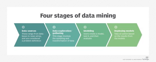
Data gathering. Relevant data for an analytics application is identified and assembled. The data may be located in different source systems, a data warehouse or a data lake, an increasingly common repository in big data environments that contain a mix of structured and unstructured data. External data sources may also be used. Wherever the data comes from, a data scientist often moves it to a data lake for the remaining steps in the process.

Data preparation. This stage includes a set of steps to get the data ready to be mined. It starts with data exploration, profiling and pre-processing, followed by data cleansing work to fix errors and other data quality issues. Data transformation is also done to make data sets consistent, unless a data scientist is looking to analyze unfiltered raw data for a particular application.

Mining the data. Once the data is prepared, a data scientist chooses the appropriate data mining technique and then implements one or more algorithms to do the mining. In machine learning applications, the algorithms typically must be trained on sample data sets to look for the information being sought before they're run against the full set of data.

Data analysis and interpretation. The data mining results are used to create analytical models that can help drive decision-making and other business actions. The data scientist or another member of a data science team also must communicate the findings to business executives and users, often through data visualization and the use of data storytelling techniques.

Types of data mining techniques

Various techniques can be used to mine data for different data science applications. Pattern recognition is a common data mining use case that's enabled by multiple techniques, as is anomaly detection, which aims to identify outlier values in data sets. Popular data mining techniques include the following types:

Association rule mining. In data mining, association rules are if-then statements that identify relationships between data elements. Support and confidence criteria are used to assess the relationships -- support measures how frequently the related elements appear in a data set, while confidence reflects the number of times an if-then statement is accurate.

Classification. This approach assigns the elements in data sets to different categories defined as part of the data mining process. Decision trees, Naive Bayes classifiers, k-nearest neighbor and logistic regression are some examples of classification methods.

Clustering. In this case, data elements that share particular characteristics are grouped together into clusters as part of data mining applications. Examples include k-means clustering, hierarchical clustering and Gaussian mixture models.

Regression. This is another way to find relationships in data sets, by calculating predicted data values based on a set of variables. Linear regression and multivariate regression are examples. Decision trees and some other classification methods can be used to do regressions, too

Data mining companies follow the procedure

[derderistuff]

My Multi_regression

Assignment 3: Test a Multiple Regression Model

This is the third assignment for the regression modeling practice course, third from a series of five courses from Data Analysis and Interpretation ministered from Wesleyan University. The previous content you can see here.

In this assignment, we have to Test a Multiple Regression Model with our data.

My response variable is the number of new cases of breast cancer in 100,000 female residents during the year 2002. My explanatory variable is the mean of sugar consumption quantity (grams per person and day) between the years 1961 and 2002.

To make the assignment of this week I have added two other explanatory variables:

Mean of the total supply of food (kilocalories / person & day) available in a country, divided by the population and 365 (the number of days in the year) between the years 1961 and 2002. The average of the mean TC (Total Cholesterol) of the female population, counted in mmol per L; (calculated as if each country has the same age composition as the world population) between the years 1980 and 2002. Note that all my explanatory variables are quantitative. Thus, I must center the variables by subtracting the mean from the data values, then the value 0 will be very close to the mean.

All of the images posted in the blog can be better view by clicking the right button of the mouse and opening the image in a new tab.

The complete program for this assignment can be download here and the dataset here.

Test a Multiple Regression Model

The first thing to do is to import the libraries and prepare the data to be used.

Test a Multiple Regression Model

The first thing to do is to import the libraries and prepare the data to be used.

In [144]:

1import numpy

2import pandas

3import matplotlib.pyplot as plt

4import statsmodels.api as sm

5import statsmodels.formula.api as smf

6import seaborn

7​

8# bug fix for display formats to avoid run time errors

9pandas.set_option('display.float_format', lambda x:'%.2f'%x)

10​

11#load the data

12data = pandas.read_csv('separatedData.csv')

13​

14# convert to numeric format

15data["breastCancer100th"] = pandas.to_numeric(data["breastCancer100th"], errors='coerce')

16data["meanSugarPerson"] = pandas.to_numeric(data["meanSugarPerson"], errors='coerce')

17data["meanFoodPerson"] = pandas.to_numeric(data["meanFoodPerson"], errors='coerce')

18data["meanCholesterol"] = pandas.to_numeric(data["meanCholesterol"], errors='coerce')

19​

20# listwise deletion of missing values

21sub1 = data[['breastCancer100th', 'meanSugarPerson', 'meanFoodPerson', 'meanCholesterol']].dropna()

The explanatory variables are centered and the first OLS Regression Test was made with only the meanSugarPerson variable.

In [146]:

1# center quantitative IVs for regression analysis

2sub1['meanSugarPerson_c'] = (sub1['meanSugarPerson'] - sub1['meanSugarPerson'].mean())

3sub1['meanFoodPerson_c'] = (sub1['meanFoodPerson'] - sub1['meanFoodPerson'].mean())

4sub1['meanCholesterol_c'] = (sub1['meanCholesterol'] - sub1['meanCholesterol'].mean())

5sub1[["meanSugarPerson_c", "meanFoodPerson_c", 'meanCholesterol_c']].describe()

6​

7# linear regression analysis

8reg1 = smf.ols('breastCancer100th ~ meanSugarPerson_c', data=sub1).fit()

9print (reg1.summary()) OLS Regression Results ============================================================================== Dep. Variable: breastCancer100th R-squared: 0.410 Model: OLS Adj. R-squared: 0.406 Method: Least Squares F-statistic: 88.34 Date: Fri, 10 Mar 2023 Prob (F-statistic): 2.99e-16 Time: 10:45:38 Log-Likelihood: -560.18 No. Observations: 129 AIC: 1124. Df Residuals: 127 BIC: 1130. Df Model: 1 Covariance Type: nonrobust ===================================================================================== coef std err t P>|t| [0.025 0.975] ------------------------------------------------------------------------------------- Intercept 37.9876 1.651 23.007 0.000 34.720 41.255 meanSugarPerson_c 0.3667 0.039 9.399 0.000 0.289 0.444 ============================================================================== Omnibus: 3.414 Durbin-Watson: 1.778 Prob(Omnibus): 0.181 Jarque-Bera (JB): 3.052 Skew: 0.291 Prob(JB): 0.217 Kurtosis: 2.522 Cond. No. 42.3 ============================================================================== Notes: [1] Standard Errors assume that the covariance matrix of the errors is correctly specified.

We can see in the OLS Regression Results that the p-value is considerably less than our alpha level of 0.05 wich tells us that we can reject the null hypothesis and concludes that the sugar consumption is significantly associated with the incidence of breast cancer cases.

The coefficient for sugar consumption is 0.3667 and the intercept is 37.9876. This means that the equation for the best line of this graph is:

breastCancer100th = 37.9876 + 0.3667 * meanSugarPerson The column P>| t | give us the p-value for our explanatory variables, association with the response variable. This p-value is 0.000 wich means that it is really small confirming the significance associated with the variables.

Other information that OLS Regression Results give to us is the R-square. This value can be interpreted in the following way: If we know the sugar consumption grams per day of a woman we can predict 41% of the variability we will see in the incidence of breast cancer cases.

After make the linear regression test, we are going to do now the polynomial regression test. For this, we have to add the polynomial second order of the meanSugarPerson variable into the scatterplot and into the regression analysis.

In [147]:

1# first order (linear) scatterplot

2scat1 = seaborn.regplot(x="meanSugarPerson", y="breastCancer100th", scatter=True, data=sub1)

3plt.xlabel('Mean of the sugar consumption between 1961 and 2002.')

4plt.ylabel('Incidence of breast cancer in 100,000 female residents during the 2002 year.')

5​

6# fit second order polynomial

7# run the 2 scatterplots together to get both linear and second order fit lines

8scat1 = seaborn.regplot(x="meanSugarPerson", y="breastCancer100th", scatter=True, order=2, data=sub1)

9plt.xlabel('Mean of the sugar consumption between 1961 and 2002.')

10plt.ylabel('Incidence of breast cancer in 100,000 female residents during the 2002 year.')

Out[147]:Text(0, 0.5, 'Incidence of breast cancer in 100,000 female residents during the 2002 year.')

In [148]:

1# quadratic (polynomial) regression analysis

2reg2 = smf.ols('breastCancer100th ~ meanSugarPerson_c + I(meanSugarPerson_c**2)', data=sub1).fit()

3print (reg2.summary()) OLS Regression Results ============================================================================== Dep. Variable: breastCancer100th R-squared: 0.430 Model: OLS Adj. R-squared: 0.421 Method: Least Squares F-statistic: 47.52 Date: Fri, 10 Mar 2023 Prob (F-statistic): 4.18e-16 Time: 10:54:56 Log-Likelihood: -557.98 No. Observations: 129 AIC: 1122. Df Residuals: 126 BIC: 1131. Df Model: 2 Covariance Type: nonrobust ============================================================================================= coef std err t P>|t| [0.025 0.975] --------------------------------------------------------------------------------------------- Intercept 34.4829 2.339 14.742 0.000 29.854 39.112 meanSugarPerson_c 0.3680 0.039 9.556 0.000 0.292 0.444 I(meanSugarPerson_c ** 2) 0.0020 0.001 2.089 0.039 0.000 0.004 ============================================================================== Omnibus: 1.821 Durbin-Watson: 1.808 Prob(Omnibus): 0.402 Jarque-Bera (JB): 1.520 Skew: 0.263 Prob(JB): 0.468 Kurtosis: 3.075 Cond. No. 3.58e+03 ============================================================================== Notes: [1] Standard Errors assume that the covariance matrix of the errors is correctly specified. [2] The condition number is large, 3.58e+03. This might indicate that there are strong multicollinearity or other numerical problems.

For the polynomial OLS Regression Results, we can see that the p-value still less than 0.05 assuming that we can reject the null hypothesis and concludes that the correlation between sugar consumption and incidence of breast cancer is significantly strong.

The coefficient for sugar consumption is 0.3680, for the polynomial sugar consumption we have a value of 0.0020 and for the intercept 34.4829. This means that the equation for the best line of this graph is:

breastCancer100th = 34.4829 + 0.3680 * meanSugarPerson + 0.0020 * meanSugarPerson²

The R-square in this scenario is slightly greater than the previous and can be interpreted as If we know the sugar consumption grams per day of a woman we can predict 43% of the variability we will see in the incidence of breast cancer cases.

After this analysis is time to add another explanatory variable, the amount of food consumption in kilocalories per day.

In [149]:

1# adding food consumption

2reg3 = smf.ols('breastCancer100th ~ meanSugarPerson_c + I(meanSugarPerson_c**2) + meanFoodPerson_c',

3 data=sub1).fit()

4print (reg3.summary()) OLS Regression Results ============================================================================== Dep. Variable: breastCancer100th R-squared: 0.653 Model: OLS Adj. R-squared: 0.645 Method: Least Squares F-statistic: 78.54 Date: Fri, 10 Mar 2023 Prob (F-statistic): 1.27e-28 Time: 10:56:09 Log-Likelihood: -525.90 No. Observations: 129 AIC: 1060. Df Residuals: 125 BIC: 1071. Df Model: 3 Covariance Type: nonrobust ============================================================================================= coef std err t P>|t| [0.025 0.975] --------------------------------------------------------------------------------------------- Intercept 33.5975 1.834 18.320 0.000 29.968 37.227 meanSugarPerson_c 0.1377 0.040 3.476 0.001 0.059 0.216 I(meanSugarPerson_c ** 2) 0.0025 0.001 3.333 0.001 0.001 0.004 meanFoodPerson_c 0.0316 0.004 8.975 0.000 0.025 0.039 ============================================================================== Omnibus: 0.058 Durbin-Watson: 1.720 Prob(Omnibus): 0.971 Jarque-Bera (JB): 0.062 Skew: 0.042 Prob(JB): 0.970 Kurtosis: 2.935 Cond. No. 3.59e+03 ============================================================================== Notes: [1] Standard Errors assume that the covariance matrix of the errors is correctly specified. [2] The condition number is large, 3.59e+03. This might indicate that there are strong multicollinearity or other numerical problems.

The OLS Regression Results demonstrates the p-value and the P>| t | for all variables lower than 0.05. We can conclude that both meanSugarPerson and meanFoodPerson are significantly associated with the incidence of new breast cancer cases.

The R-square increased considerably from 43% to 65.3%.

Thereafter, as the meanFoodPerson improved the study, let’s try to add the cholesterol in blood variable.

In [150]:

1# adding mean cholesterol

2reg4 = smf.ols('breastCancer100th ~ meanSugarPerson_c + I(meanSugarPerson_c**2) + meanCholesterol_c',

3 data=sub1).fit()

4print (reg4.summary()) OLS Regression Results ============================================================================== Dep. Variable: breastCancer100th R-squared: 0.728 Model: OLS Adj. R-squared: 0.722 Method: Least Squares F-statistic: 111.6 Date: Fri, 10 Mar 2023 Prob (F-statistic): 3.40e-35 Time: 11:01:39 Log-Likelihood: -510.23 No. Observations: 129 AIC: 1028. Df Residuals: 125 BIC: 1040. Df Model: 3 Covariance Type: nonrobust ============================================================================================= coef std err t P>|t| [0.025 0.975] --------------------------------------------------------------------------------------------- Intercept 32.7510 1.629 20.111 0.000 29.528 35.974 meanSugarPerson_c 0.0165 0.040 0.410 0.683 -0.063 0.096 I(meanSugarPerson_c ** 2) 0.0029 0.001 4.465 0.000 0.002 0.004 meanCholesterol_c 45.7660 3.909 11.709 0.000 38.030 53.502 ============================================================================== Omnibus: 5.132 Durbin-Watson: 1.947 Prob(Omnibus): 0.077 Jarque-Bera (JB): 5.067 Skew: -0.316 Prob(JB): 0.0794 Kurtosis: 3.736 Cond. No. 8.65e+03 ============================================================================== Notes: [1] Standard Errors assume that the covariance matrix of the errors is correctly specified. [2] The condition number is large, 8.65e+03. This might indicate that there are strong multicollinearity or other numerical problems.

#######When we add the meanCholesterol variable to the multiple regression tests, we can see that this variable made the meanSugarPerson p-value get increased over than 0.5, assuming that the meanCholesterol is a confounding variable for this work.

Q-Q Plot

In [154]:

1#Q-Q plot for normality

2fig4 = sm.qqplot(reg3.resid, line='r')

3plt.show(fig4)

The qqplot for our regression model shows that the residuals generally follow a straight line, but deviate at the lower and higher quantiles. This indicates that our residuals did not follow perfect normal distribution meaning that the curvilinear association that we observed in our scatter plot may not be fully estimated by the quadratic sugar consumption.

In [155]:

1# simple plot of residuals

2stdres = pandas.DataFrame(reg3.resid_pearson)

3plt.plot(stdres, 'o', ls='None')

4l = plt.axhline(y=0, color='r')

5plt.ylabel('Standardized Residual')

6plt.xlabel('Observation Number')

Out[155]:Text(0.5, 0, 'Observation Number')

“The standardized residuals are simply the residual values transformed to have a mean of zero and a standard deviation of one. This transformation is called normalizing or standardizing the values so that they fit a standard normal distribution. In a standard normal distribution 68% of the observations are expected to fall within one standard deviation of the mean. So between -1 and 1 standard deviations. And 95% of the observations are expected to fall within 2 standard deviations of the mean.

With the standard normal distribution, we would expect 95% of the values of the residuals to fall between two standard deviations of the mean. Residual values that are more than two standard deviations from the mean in either direction, are a warning sign that we may have some outliers. However, there are no observations that have three or more standard deviations from the mean. So we do not appear to have any extreme outliers.

In terms of evaluating the overall fit of the model, there’s some other rules of thumb that you can use to determine how well your model fits the data based on the distribution of the residuals. If more than 1% of our observations has standardized residuals with an absolute value greater than 2.5, or more than 5% have an absolute value of greater than or equal to 2, then there is evidence that the level of error within our model is unacceptable. That is the model is a fairly poor fit to the observed data.”

In this work, only 1 point is exceeded an absolute value of 2.5 representing less than 1% and there are 6 points (4.65%) that are greater than or equal to an absolute value of 2.0. This suggests that the model is good.

additional regression diagnostic plots

In [156]:

1# additional regression diagnostic plots

2fig2 = plt.figure(figsize=(12,8))

3fig2 = sm.graphics.plot_regress_exog(reg3, "meanFoodPerson_c", fig=fig2)

4plt.show(fig2)

he plot in the upper right hand corner shows the residuals for each observation at different values of mean food consumption. There’s not a clearly pattern on it, as there is points all over the graph, we can assume that model predict food consumption kilocalories as well for countries that have either high or low incidence of breast cancer new cases.

To take a look at the contribution of each individual explanatory variable to model fit we analysis the partial regression residual plot (the third plot). It attempts to show the effect of adding meanFoodPerson as an additional explanatory variable to the model. Given that one or more explanatory variables are already in the model. This plot demonstrates the relationship between the response variable and specific explanatory variable, after controlling for the other explanatory variables. We can see that the meanFoodPerson has a linear pattern meaning that it meets the linearity assumption in the multiple regression.

Leverage Plot

In [157]:

1# leverage plot

2fig3=sm.graphics.influence_plot(reg3, size=8)

3plt.show(fig3)

“Finally, we can examine a leverage plot to identify observations that have an unusually large influence on the estimation of the predicted value of the response variable, mean of sugar consumption grams per day, or that are outliers, or both.

The leverage of an observation can be thought of in terms of how much the predicted scores for the other observations would differ if the observations in question were not included in the analysis. The leverage always takes on values between zero and one. A point with zero leverage has no effect on the regression model. And outliers are observations with residuals greater than 2 or less than -2.”

One of the first things we see in the leverage plot is that we have a few outliers, contents that have residuals greater than 2 or less than -2. We’ve already identified some of these outliers in some of the other plots we’ve looked at, but this plot also tells us that these outliers have small or close to zero leverage values, meaning that although they are outlying observations, they do not have an undue influence on the estimation of the regression model. On the other hand, we see that there are a few cases with higher than average leverage. But one in particular is more obvious in terms of having an influence on the estimation of the predicted value of sugar consumption per day. This observation has a high leverage but is not an outlier. We don’t have any observations that are both high leverage and outliers.

In [ ]:

1​

[tchaikovskym]

Me: oh yeah I have 4 months to finish my thesis and I will leave the data analysis last when I will be on vacation and will be able to fully go in my red string detective board mode

Thesis advisor: hey. Do you want to go to a conference? You have to have some results and analysis to be able to write an abstract by the end of next month

Me: sure! (What the fuck do I do with my data there are so many its just a month I can do so much but I'm an impostor I only had two courses in statitistics I done even know how to do multiple factor regression I mean I do if I look it up but everything I do is false I don't understand a thing in this world oh my god why am I doing this maybe they won't even accept me in t