#catplotting
Explore tagged Tumblr posts
Text
Data Analysis tools: Module 2. chi square test of independence
Results
Null hypothesis that there is no difference in the mean of the quantitative variable “femaleemployrate “ across groups for “incomeperperson”
The explantory variable is the income per person in 5 levels (poor, low class, midle class, upper class, rich) and the respond variable is the Female employ rate considering 2 levels ( between 0% and 40% and between 40% and 100%)
distribution for income per person splits into 6 groups and creating a new variable income as categorical variable
poor 80
low class 46
midle class 39
upper class 22
rich 3
NaN 23
Name: income, dtype: int64
distribution for femaleemployrate splits into 2 groups (employ rate between 0% & 40% =0, 40% & 100%=1) and creating a new variable Femaleemploy as categorical variable
0 52
1 126
NaN 35
Name: Femaleemploy, dtype: int64
table of observed counts
income poor low class midle class upper class
Femaleemploy
0 18 14 14 1
1 56 25 18 20
table of observed counts in %
income poor low class midle class upper class
Femaleemploy
0 0.243243 0.358974 0.437500 0.047619
1 0.756757 0.641026 0.562500 0.952381
chi-square value, p value, expected counts
(11.181092289173819, 0.010785880920040842, 3, array([[20.95180723, 11.04216867, 9.06024096, 5.94578313],
[53.04819277, 27.95783133, 22.93975904, 15.05421687]]))
income poor low class midle class upper class
Femaleemploy
0 18 14 14 1
1 56 25 18 20
C:\ProgramData\Anaconda3\lib\site-packages\seaborn\categorical.py:3717: UserWarning: The `factorplot` function has been renamed to `catplot`. The original name will be removed in a future release. Please update your code. Note that the default `kind` in `factorplot` (`'point'`) has changed `'strip'` in `catplot`.
warnings.warn(msg)
Out[42]: Text(6.799999999999997, 0.5, 'Female employ rate')
runfile('G:/QMM/01 Productos/02 USS/04 USS5/python/prueba6-bis.py', wdir='G:/QMM/01 Productos/02 USS/04 USS5/python')
Null hypothesis that there is no difference in the mean of the quantitative variable “femaleemployrate “ across groups for “incomeperperson”
The explantory variable is the income per person in 5 levels (poor, low class, midle class, upper class, rich) and the respond variable is the Female employ rate considering 2 levels ( between 0% and 40% and between 40% and 100%)
distribution for income per person splits into 6 groups and creating a new variable income as categorical variable
poor 54
low class 26
midle class 46
upper class 39
rich 22
NaN 26
Name: income, dtype: int64
distribution for femaleemployrate splits into 2 groups (employ rate between 0% & 40% =0, 40% & 100%=1) and creating a new variable Femaleemploy as categorical variable
0 52
1 126
NaN 35
Name: Femaleemploy, dtype: int64
table of observed counts
income poor low class midle class upper class rich
Femaleemploy
0 11 7 14 14 1
1 41 15 25 18 20
table of observed counts in %
income poor low class midle class upper class rich
Femaleemploy
0 0.211538 0.318182 0.358974 0.437500 0.047619
1 0.788462 0.681818 0.641026 0.562500 0.952381
chi-square value, p value, expected counts
(12.047322395704303, 0.01700281130675494, 4, array([[14.72289157, 6.22891566, 11.04216867, 9.06024096, 5.94578313],
[37.27710843, 15.77108434, 27.95783133, 22.93975904, 15.05421687]]))
income poor low class midle class upper class rich
Femaleemploy
0 11 7 14 14 1
1 41 15 25 18 20
Group poor-low class
table of observed counts
income2 low class poor
Femaleemploy
0 7 11
1 15 41
table of observed counts in %
income2 low class poor
Femaleemploy
0 0.318182 0.211538
1 0.681818 0.788462
chi-square value, p value, expected counts
(0.4636422605172603, 0.49592665933844127, 1, array([[ 5.35135135, 12.64864865],
[16.64864865, 39.35135135]]))
Group poor-midle class
table of observed counts
income3 midle class poor
Femaleemploy
0 14 11
1 25 41
table of observed counts in %
income3 midle class poor
Femaleemploy
0 0.358974 0.211538
1 0.641026 0.788462
chi-square value, p value, expected counts
(1.7476136363636368, 0.18617701296552153, 1, array([[10.71428571, 14.28571429],
[28.28571429, 37.71428571]]))
Group poor-upper class
table of observed counts
income4 poor upper class
Femaleemploy
0 11 14
1 41 18
table of observed counts in %
income4 poor upper class
Femaleemploy
0 0.211538 0.437500
1 0.788462 0.562500
chi-square value, p value, expected counts
(3.8179204693611464, 0.05070713462718701, 1, array([[15.47619048, 9.52380952],
[36.52380952, 22.47619048]]))
Group poor- rich
table of observed counts
income5 poor rich
Femaleemploy
0 11 1
1 41 20
table of observed counts in %
income5 poor rich
Femaleemploy
0 0.211538 0.047619
1 0.788462 0.952381
chi-square value, p value, expected counts
(1.8544659745991714, 0.17326486722177523, 1, array([[ 8.54794521, 3.45205479],
[43.45205479, 17.54794521]]))
Group low class-midle class
table of observed counts
income6 low class midle class
Femaleemploy
0 7 14
1 15 25
table of observed counts in %
income6 low class midle class
Femaleemploy
0 0.318182 0.358974
1 0.681818 0.641026
chi-square value, p value, expected counts
(0.001713911088911098, 0.9669774837195514, 1, array([[ 7.57377049, 13.42622951],
[14.42622951, 25.57377049]]))
Group low class-upper class
table of observed counts
income7 low class upper class
Femaleemploy
0 7 14
1 15 18
table of observed counts in %
income7 low class upper class
Femaleemploy
0 0.318182 0.437500
1 0.681818 0.562500
chi-square value, p value, expected counts
(0.3596148170011807, 0.5487202341134262, 1, array([[ 8.55555556, 12.44444444],
[13.44444444, 19.55555556]]))
Group low class-rich
table of observed counts
income8 low class rich
Femaleemploy
0 7 1
1 15 20
table of observed counts in %
income8 low class rich
Femaleemploy
0 0.318182 0.047619
1 0.681818 0.952381
chi-square value, p value, expected counts
(3.5608128478664187, 0.059158762972845974, 1, array([[ 4.09302326, 3.90697674],
[17.90697674, 17.09302326]]))
Group midle class-upperclass
table of observed counts
income9 midle class upper class
Femaleemploy
0 14 14
1 25 18
table of observed counts in %
income9 midle class upper class
Femaleemploy
0 0.358974 0.437500
1 0.641026 0.562500
chi-square value, p value, expected counts
(0.1845768844769572, 0.667469088625999, 1, array([[15.38028169, 12.61971831],
[23.61971831, 19.38028169]]))
Group midle class-rich
table of observed counts
income10 midle class rich
Femaleemploy
0 14 1
1 25 20
table of observed counts in %
income10 midle class rich
Femaleemploy
0 0.358974 0.047619
1 0.641026 0.952381
chi-square value, p value, expected counts
(5.4945054945054945, 0.01907632210177841, 1, array([[ 9.75, 5.25],
[29.25, 15.75]]))
Group upper class-rich
table of observed counts
income11 rich upper class
Femaleemploy
0 1 14
1 20 18
table of observed counts in %
income11 rich upper class
Femaleemploy
0 0.047619 0.437500
1 0.952381 0.562500
chi-square value, p value, expected counts
(7.673854558270678, 0.005602664662587936, 1, array([[ 5.94339623, 9.05660377],
[15.05660377, 22.94339623]]))
0 notes
Text
Data Visualization for the GapMinder Dataset
I have worked on selecting a research topic that can be improved on due to the tasks to be performed on the dataset, creating my own dataset, examining the frequency distributions of the observations, and also data management on the dataset so far.
This post is to explain the visualization processes taken on the dataset and the results gotten.
Summary of Results
‘incomeperperson’ variable is skewed to the right with value of 8740.966+/-14262.809 on the average. The variable has a large variability.
‘urbanrate’ variable is roughly bimodal with 56.769+/-23.845 value on the average. The variable is low in variability.
‘relectricperperson’ variable is skewed to the right with value 1173.179+/-1681.440 on the average. The variable has large variability.
‘relectricperperson’ is positively related to ‘incomeperperson’ and ‘urbanrate’ respectively.
Outline of Code Cells
The code is just addition to what has been seen in the previous GapMinder posts, so i will just add the visualization code lines.
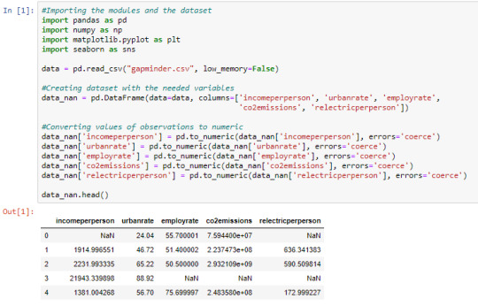
Cell 1: Import modules needed, load dataset, create a dataset with variables you need, convert its observation values to numeric
Cell 2: Replacing missing data with NaN using np.nan
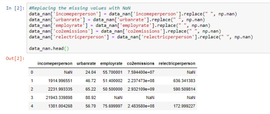
From cell 1, it is noticed that once the observations are converted to numeric, the missing data automatically become NaN. This is just another way of doing it.
Cell 3: Visualizing ‘incomeperperson’ using the describe() function and graphing a univariate distplot
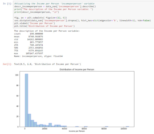
From the output, we can say the ‘incomeperperson’ is skewed to the right. On the average, ‘incomeperperson’ for each country is 8740.966+/-14262.809. This wide range causes large variability in the variable.
Cell 4: Visualizing ‘urbanrate’ using the describe() function and graphing a univariate distplot
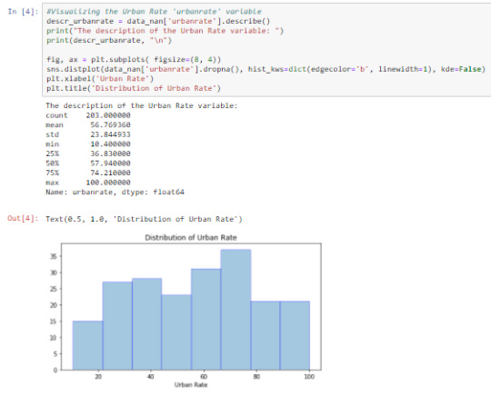
The output shows a roughly bimodal graph. On the average, ‘urbanrate’ for each country is 56.769+/-23.845. The range is not so wide making variability low.
Cell 5: Visualizing ‘relectricperperson’ using the describe() function and graphing a univariate distplot
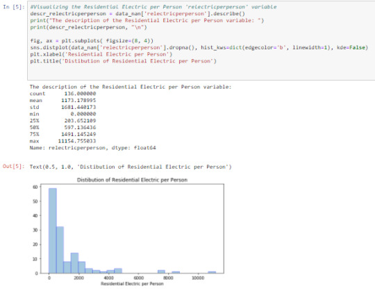
From the output, ‘relectricperperson’ is skewed to the right. On the average, ‘relectricperperson’ takes value 1173.179+/-1681.440. This wide range causes large variability in the variable graph.
Cell 6: Visualizing the relationship between ‘incomeperperson’ and ‘relectricperperson’ by graphing a bi-variate scatterplot
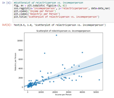
The regression line on the graph shows a positive relationship between these variables. But the scatterplot shows a weak relationship between them. The ‘relecticperperson’ values are clustered at ‘incomeperperson’<10000, and scattered all over for the remaining ranges.
Cell 7: Visualizing the relationship between ‘incomeperperson’ and ‘relectricperperson’ by graphing a bi-variate barchart
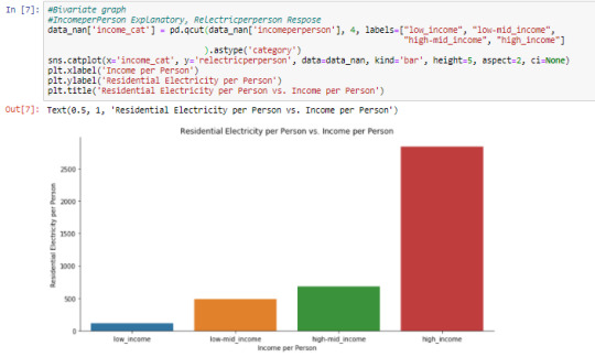
Using the data management process in the ‘Data Management of the GapMinder dataset’ post, ‘incomeperperson’ was categorized into 4 using quartiles as ‘income_cat’. ‘relectricperperson’ is plotted against ‘income_cat’, and ‘relectricperperson’ increases as ‘income_cat’ increases, with high_income category having the most residential electricity per person and low_income category having the least.
Cell 8: Visualizing the relationship between ‘urbanrate’ and ‘relectricperperson’ by graphing a bi-variate scatterplot
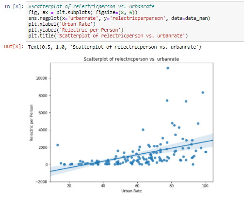
The regression line on graph shows, positive relationship between the two variables. The scatterplot shows a stronger relationship between the variables than that in Cell 6.
Cell 9: Visualizing the relationship between ‘urbanrate’ and ‘relectricperperson’ by graphing a bi-variate barchart
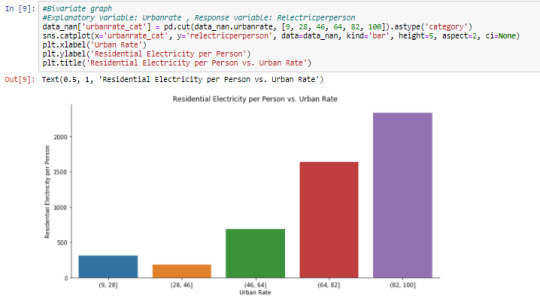
Using ‘urbanrate_cat’ created in the ‘Data Management of the GapMinder dataset’ post, having a range interval of 18 for each category. ‘relectricperperson’ is plotted against ‘urbanrate_cat’. The graph shows a slight decrease in the (28, 46] category then increase in ‘relecticperperson’ has we move up the other ‘urbanrate_cat’ categories.
Cell 10: Dataset after the data management and visualization processes

Things to note:
factorplot has been changed to catplot in seaborn
The size argument in factorplot has been changed to height
When handling categorical data, you can let python by calling the astype(‘category’) on your dataset
1 note
·
View note
Text
Hypothesis Testing and Chi Square Test of Independence
This assignment aims to directly test my hypothesis by evaluating, based on a sample of 4946 U.S. which resides in South region(REGION) aged between 25 to 40 years old(subsetc1), my research question with a goal of generalizing the results to the larger population of NESARC survey, from where the sample has been drawn. Therefore, I statistically assessed the evidence, provided by NESARC codebook, in favor of or against the association between Cigars smoked status and fear/avoidance of heights, in U.S. population in the South region. As a result, in the first place I used crosstab function, in order to produce a contingency table of observed counts and percentages for fear/avoidance of heights. Next, I wanted to examine if the Cigars smoked status (1= Yes or 2=no) variable ‘S3AQ42′, which is a 2-level categorical explanatory variable, is correlated with fear/avoidance of heights (’S8Q1A2′), which is a categorical response variable. Thus , I ran Chi-square Test of Independence(C->C) and calculated the χ-squared values and the associated p-values for our specific conditions, so that null and alternate hypothesis are specified. In addition, in order visualize the association between frequency of cannabis use and depression diagnosis, I used catplot function to produce a bivariate graph. Furthermore, I used crosstab function once again and tested the association between the frequency of cannabis use (’S3BD5Q2E’), which is a 10-level categorical explanatory variable. In this case, for my second Test of Independence (C->C), after measuring the χ-square value and the p-value, in order to determine which frequency groups are different from the others, I performed a post hoc test, using Bonferroni Adjustment approach, since my explanatory variable has more than 2 levels. In this case of ten groups, I actually need to conduct 45 pair wise comparisons, but in fact I examined indicatively two and compared their p-values with the Bonferroni adjusted p-value, which is calculated by dividing p = 0.05 by 45. By this way it is possible to identify the situations where null hypothesis can be safely rejected without making an excessive type 1 error. For the code and the output I used Jupyter Notebook(IDE).
PROGRAM:
import pandas as pd
import numpy as np
import scipy.stats
import seaborn
import matplotlib.pyplot as plt
data = pd.read_csv('nesarc_pds.csv',low_memory=False)
data['AGE'] = pd.to_numeric(data['AGE'],errors='coerce')
data['REGION'] = pd.to_numeric(data['REGION'],errors='coerce')
data['S3AQ42'] = pd.to_numeric(data['S3AQ42'],errors='coerce')
data['S3BQ1A5'] = pd.to_numeric(data['S3BQ1A5'],errors='coerce')
data['S8Q1A2'] = pd.to_numeric(data['S8Q1A2'],errors='coerce')
data['S3BD5Q2E'] = pd.to_numeric(data['S3BD5Q2E'],errors='coerce')
data['MAJORDEP12'] = pd.to_numeric(data['MAJORDEP12'],errors='coerce')
subset1 = data[(data['AGE']>=25) & (data['AGE']<=40) & (data['REGION']==3)]
subsetc1 = subset1.copy()
subset2 = data[(data['AGE']>=18) & (data['AGE']<=30) & (data['S3BQ1A5']==1)]
subsetc2 = subset2.copy()
subsetc1['S3AQ42'] = subsetc1['S3AQ42'].replace(9,np.NaN)
subsetc1['S8Q1A2'] = subsetc1['S8Q1A2'].replace(9,np.NaN)
subsetc2['S3BD5Q2E'] = subsetc2['S3BD5Q2E'].replace(99,np.NaN)
cont1 = pd.crosstab(subsetc1['S8Q1A2'],subsetc1['S3AQ42'])
print(cont1)
colsum = cont1.sum()
contp = cont1/colsum
print(contp)
print ('Chi-square value, p value, expected counts, for fear/avoidance of heights within Cigar smoked status')
chsq1 = scipy.stats.chi2_contingency(cont1)
print(chsq1)
cont2 = pd.crosstab(subsetc2['MAJORDEP12'],subsetc2['S3BD5Q2E'])
print(cont2)
colsum = cont2.sum()
contp2 = cont2/colsum
print(contp2)
print('Chi-square value, p value, expected counts, for major depression within cannabis use status')
chsq2 = scipy.stats.chi2_contingency(cont2)
print(chsq2)
recode = {1:10,2:9,3:8,4:7,5:6,6:5,7:4,8:3,9:2,10:1}
subsetc2['CUFREQ'] = subsetc2['S3BD5Q2E'].map(recode)
subsetc2['CUFREQ'] = subsetc2['CUFREQ'].astype('category')
subsetc2['CUFREQ'] = subsetc2['CUFREQ'].cat.rename_categories(['Once a year','2 times a year','3 to 6 times a year','7 to 11 times a year','Once a month','2 to 3 times a month','1 to 2 times a week','3 to 4 times a week','Nearly Everyday','Everyday'])
plt.figure(figsize=(16,8))
ax1 = seaborn.catplot(x='CUFREQ',y='MAJORDEP12', data=subsetc2, kind="bar", ci=None)
ax1.set_xticklabels(rotation=40, ha="right")
plt.xlabel('Frequency of cannabis use')
plt.ylabel('Proportion of Major Depression')
plt.show()
recode={1:1,9:9}
subsetc2['COMP1v9'] = subsetc2['S3BD5Q2E'].map(recode)
cont3 = pd.crosstab(subsetc2['MAJORDEP12'],subsetc2['COMP1v9'])
print(cont3)
colsum = cont3.sum()
contp3 = cont3/colsum
print(contp3)
print('Chi-square value, p value, expected counts, for major depression within pair comparisons of frequency groups -Everyday- and -2 times a year-')
chsq3 = scipy.stats.chi2_contingency(cont3)
print(chsq3)
recode={4:4,9:9}
subsetc2['COMP4v9'] = subsetc2['S3BD5Q2E'].map(recode)
cont4 = pd.crosstab(subsetc2['MAJORDEP12'],subsetc2['COMP4v9'])
print(cont4)
colsum = cont4.sum()
contp4 = cont4/colsum
print(contp4)
print('Chi-square value, p value, expected counts, for major depression within pair comparisons of frequency groups -1 to 2 times a week- and -2 times a year-')
chsq4 = scipy.stats.chi2_contingency(cont4)
print(chsq4)
*******************************************************************************************
OUTPUT:

When examining the patterns of association between fear/avoidance of heights (categorical response variable) and Cigars use status (categorical explanatory variable), a chi-square test of independence revealed that among aged between 25 to 40 in the South region(subsetc1), those who were Cigars users, were more likely to have the fear/avoidance of heights(26%), compared to the non-users(20%), X2=0.26,1 df, p=0.6096. As a result, since our p-value is not smaller than 0.05(Level of Significance), the data does not provide enough evidence against the null hypothesis. Thus, we accept the null hypothesis , which indicates that there is no positive correlation between Cigar users and fear/avoidance of heights.
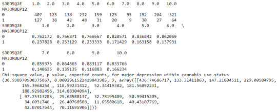
A Chi Square test of independence revealed that among cannabis users aged between 18 to 30 years old (susbetc2), the frequency of cannabis use (explanatory variable collapsed into 10 ordered categories) and past year depression diagnosis (response binary categorical variable) were significantly associated, X2 = 30.99,9 df, p=0.00029.
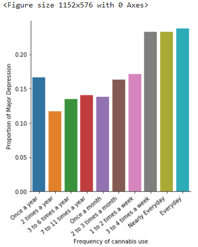
In the bivariate graph(C->C) presented above, we can see the correlation between frequency of cannabis use (explanatory variable) and major depression diagnosis in the past year (response variable). Obviously, we have a left-skewed distribution, which indicates that the more an individual (18-30) smoked cannabis, the better were the cases to have experienced depression in the last 12 months.

The post hoc comparison (Bonferroni Adjustment) of rates of major depression by the pair of “Every day” and “2 times a year” frequency categories, revealed that the p-value is 0.00019 and the percentages of major depression diagnosis for each frequency group are 23.7% and 11.6% respectively. As a result, since the p-value is smaller than the Bonferroni adjusted p-value (adj p-value = 0.05 / 45 = 0.0011>0.00019), we can assume that these two rates are significantly different from one another. Therefore, we reject the null hypothesis and accept the alternate.

Similarly, the post hoc comparison (Bonferroni Adjustment) of rates of major depression by the pair of "1 or 2 times a week” and “2 times a year” frequency categories, indicated that the p-value is 0.107 and the proportions of major depression diagnosis for each frequency group are 17.1% and 11.6% respectively. As a result, since the p-value is larger than the Bonferroni adjusted p-value (adj p-value = 0.05 / 45 = 0.107>0.0011), we can assume that these two rates are not significantly different from one another. Therefore, we accept the null hypothesis.
1 note
·
View note
Photo

Bongo plotting how he's going to take down the evil tulips... #catplotting #evilgenius #bongo #zappo #cats #revenge
0 notes
Text
Testing the relationship between Tree diameter and sidewalk with roots in stone as a moderator
I got my Dataset from kaggle: https://www.kaggle.com/datasets/yash16jr/tree-census-2015-in-nyc-cleaned
My goal is to check if there is the tree diameter is influenced by it's location on the sidewalk and to use roots in Stone as a moderator variable to check this
```python
import pandas as pd
import statsmodels.formula.api as smf
import seaborn as sb
import matplotlib.pyplot as plt
data = pd.read_csv('tree_census_processed.csv', low_memory=False)
print(data.head(0))
```
Empty DataFrame
Columns: [tree_id, tree_dbh, stump_diam, curb_loc, status, health, spc_latin, steward, guards, sidewalk, problems, root_stone, root_grate, root_other, trunk_wire, trnk_light, trnk_other, brch_light, brch_shoe, brch_other]
Index: []
```python
model1 = smf.ols(formula='tree_dbh ~ C(sidewalk)', data=data).fit()
print (model1.summary())
```
OLS Regression Results
==============================================================================
Dep. Variable: tree_dbh R-squared: 0.063
Model: OLS Adj. R-squared: 0.063
Method: Least Squares F-statistic: 4.634e+04
Date: Mon, 20 Mar 2023 Prob (F-statistic): 0.00
Time: 10:42:07 Log-Likelihood: -2.4289e+06
No. Observations: 683788 AIC: 4.858e+06
Df Residuals: 683786 BIC: 4.858e+06
Df Model: 1
Covariance Type: nonrobust
===========================================================================================
coef std err t P>|t| [0.025 0.975]
-------------------------------------------------------------------------------------------
Intercept 14.8589 0.020 761.558 0.000 14.821 14.897
C(sidewalk)[T.NoDamage] -4.9283 0.023 -215.257 0.000 -4.973 -4.883
==============================================================================
Omnibus: 495815.206 Durbin-Watson: 1.474
Prob(Omnibus): 0.000 Jarque-Bera (JB): 81727828.276
Skew: 2.589 Prob(JB): 0.00
Kurtosis: 56.308 Cond. No. 3.59
==============================================================================
Notes:
[1] Standard Errors assume that the covariance matrix of the errors is correctly specified.
Now i get the data ready to do the moderation variable check after that i check the mean and the standard deviation
```python
sub1 = data[['tree_dbh', 'sidewalk']].dropna()
print(sub1.head(1))
print ("\nmeans for tree_dbh by sidewalk")
mean1= sub1.groupby('sidewalk').mean()
print (mean1)
print ("\nstandard deviation for mean tree_dbh by sidewalk")
st1= sub1.groupby('sidewalk').std()
print (st1)
```
tree_dbh sidewalk
0 3 NoDamage
means for tree_dbh by sidewalk
tree_dbh
sidewalk
Damage 14.858948
NoDamage 9.930601
standard deviation for mean WeightLoss by Diet
tree_dbh
sidewalk
Damage 9.066262
NoDamage 8.193949
To better understand these Numbers I visualize them with a catplot.
```python
sb.catplot(x="sidewalk", y="tree_dbh", data=data, kind="bar", errorbar=None)
plt.xlabel('Sidewalk')
plt.ylabel('Mean of tree dbh')
```
Text(13.819444444444445, 0.5, 'Mean of tree dbh')


its possible to say that there is a diffrence in diameter by the state of the sidewalk now i will check if there is a effect of the roots penetrating stone.
```python
sub2=sub1[(data['root_stone']=='No')]
print ('association between tree_dbh and sidewalk for those whose roots have not penetrated stone')
model2 = smf.ols(formula='tree_dbh ~ C(sidewalk)', data=sub2).fit()
print (model2.summary())
```
association between tree_dbh and sidewalk for those using Cardio exercise
OLS Regression Results
==============================================================================
Dep. Variable: tree_dbh R-squared: 0.024
Model: OLS Adj. R-squared: 0.024
Method: Least Squares F-statistic: 1.323e+04
Date: Mon, 20 Mar 2023 Prob (F-statistic): 0.00
Time: 10:58:36 Log-Likelihood: -1.8976e+06
No. Observations: 543789 AIC: 3.795e+06
Df Residuals: 543787 BIC: 3.795e+06
Df Model: 1
Covariance Type: nonrobust
===========================================================================================
coef std err t P>|t| [0.025 0.975]
-------------------------------------------------------------------------------------------
Intercept 12.3776 0.024 506.657 0.000 12.330 12.426
C(sidewalk)[T.NoDamage] -3.1292 0.027 -115.012 0.000 -3.183 -3.076
==============================================================================
Omnibus: 455223.989 Durbin-Watson: 1.544
Prob(Omnibus): 0.000 Jarque-Bera (JB): 130499322.285
Skew: 3.146 Prob(JB): 0.00
Kurtosis: 78.631 Cond. No. 4.34
==============================================================================
Notes:
[1] Standard Errors assume that the covariance matrix of the errors is correctly specified.
There is still a significant association between them.
Now i check for those whose roots have not penetrated stone.
```python
sub3=sub1[(data['root_stone']=='Yes')]
print ('association between tree_dbh and sidewalk for those whose roots have not penetrated stone')
model3 = smf.ols(formula='tree_dbh ~ C(sidewalk)', data=sub3).fit()
print (model3.summary())
```
association between tree_dbh and sidewalk for those whose roots have not penetrated stone
OLS Regression Results
==============================================================================
Dep. Variable: tree_dbh R-squared: 0.026
Model: OLS Adj. R-squared: 0.026
Method: Least Squares F-statistic: 3744.
Date: Mon, 20 Mar 2023 Prob (F-statistic): 0.00
Time: 11:06:21 Log-Likelihood: -5.0605e+05
No. Observations: 139999 AIC: 1.012e+06
Df Residuals: 139997 BIC: 1.012e+06
Df Model: 1
Covariance Type: nonrobust
===========================================================================================
coef std err t P>|t| [0.025 0.975]
-------------------------------------------------------------------------------------------
Intercept 18.0541 0.031 574.681 0.000 17.993 18.116
C(sidewalk)[T.NoDamage] -2.9820 0.049 -61.186 0.000 -3.078 -2.886
==============================================================================
Omnibus: 72304.550 Durbin-Watson: 1.493
Prob(Omnibus): 0.000 Jarque-Bera (JB): 3838582.479
Skew: 1.739 Prob(JB): 0.00
Kurtosis: 28.416 Cond. No. 2.47
==============================================================================
Notes:
[1] Standard Errors assume that the covariance matrix of the errors is correctly specified.
There is still a significant association between them.
I visualize the means now
```python
print ("means for tree_dbh by sidewalk A vs. B for Roots not in Stone")
m3= sub2.groupby('sidewalk').mean()
print (m3)
sb.catplot(x="sidewalk", y="tree_dbh", data=sub2, kind="bar", errorbar=None)
plt.xlabel('Sidewalk Damage')
plt.ylabel('Tree Diameter at breast height')
```
means for tree_dbh by sidewalk A vs. B for Roots not in Stone
tree_dbh
sidewalk
Damage 12.377623
NoDamage 9.248400
Text(13.819444444444445, 0.5, 'Tree Diameter at breast height')


```python
print ("Means for tree_dbh by sidewalk A vs. B for Roots in Stone")
m4 = sub3.groupby('sidewalk').mean()
print (m4)
sb.catplot(x="sidewalk", y="tree_dbh", data=sub3, kind="bar", errorbar=None)
plt.xlabel('Sidewalk Damage')
plt.ylabel('Tree Diameter at breast height')
```
Means for tree_dbh by sidewalk A vs. B for Roots in Stone
tree_dbh
sidewalk
Damage 18.054102
NoDamage 15.072114
Text(0.5694444444444446, 0.5, 'Tree Diameter at breast height')

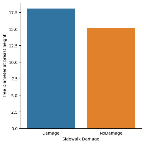
You can definetly see that there is a diffrence in overall diameter as well as its distributions among sidewalk damage an no sidewalk damage.
Therefore you can say that Roots in stone is a good moderator variable and the null hypothesis can be rejected.
0 notes
Text
Análisis tamaño Cráter en Marte
Les comparto mi código
import seaborn import pandas import matplotlib.pyplot as plt
data = pandas.read_csv('marscrater_pds.csv', low_memory=False)
data['LATITUDE_CIRCLE_IMAGE']=pandas.to_numeric(data['LATITUDE_CIRCLE_IMAGE']) data['LONGITUDE_CIRCLE_IMAGE']=pandas.to_numeric(data['LONGITUDE_CIRCLE_IMAGE']) data['DIAM_CIRCLE_IMAGE']=pandas.to_numeric(data['DIAM_CIRCLE_IMAGE']) data['NUMBER_LAYERS']=pandas.to_numeric(data['NUMBER_LAYERS']) fre_DIAM_CIRCLE_IMAGE=data["DIAM_CIRCLE_IMAGE"].value_counts(sort=False,dropna=False)
Sub1_DIAM_CIRCLE_IMAGE=data[(data['DIAM_CIRCLE_IMAGE']>=0) & (data['DIAM_CIRCLE_IMAGE']<=70000)] print(Sub1_DIAM_CIRCLE_IMAGE," Layers 1")
Sub1_DIAM_CIRCLE_IMAGE['DIAM_CIRCLE_IMAGE'] = pandas.cut(Sub1_DIAM_CIRCLE_IMAGE.NUMBER_LAYERS,[0, 1, 2, 3, 4]) Cut_x_num_layers = Sub1_DIAM_CIRCLE_IMAGE['DIAM_CIRCLE_IMAGE'].value_counts(sort=False, dropna=True) print(Cut_x_num_layers)
Clasifico los grupos por nombre del crater
print (pandas.crosstab(Sub1_DIAM_CIRCLE_IMAGE['DIAM_CIRCLE_IMAGE'],Sub1_DIAM_CIRCLE_IMAGE['CRATER_NAME']))
Definicón de variables categoricas para plotear en python
Sub1_DIAM_CIRCLE_IMAGE['CRATER_NAME'] =Sub1_DIAM_CIRCLE_IMAGE['CRATER_NAME'].astype('category') #Definición de la variable categoría plot1=seaborn.countplot(x="NUMBER_LAYERS", data=Sub1_DIAM_CIRCLE_IMAGE) plot1.plt.title ('Cantidad de Capas registradas') plot1.plt.xlabel('Layer') plot1.plt.ylabel('Cantidad layers')
Relación de las variables con la categoria establecida
plot2=seaborn.regplot(x='DIAM_CIRCLE_IMAGE', y = 'LATITUDE_CIRCLE_IMAGE', fit_reg = False, data=data) plot2.plt.title ('Relación de diametro del crater con la latitud de marte') plot2.plt.xlabel('Diametro del crater') plot2.plt.ylabel('Latitud')
plot3=seaborn.regplot(x='DIAM_CIRCLE_IMAGE', y = 'LONGITUDE_CIRCLE_IMAGE', fit_reg = False, data=data) plot3.plt.title ('Relación de diametro del crater con la longitud de marte') plot3.plt.xlabel('Diametro del crater') plot3.plt.ylabel('Longitud')
plot4=seaborn.regplot(x='DIAM_CIRCLE_IMAGE', y = 'NUMBER_LAYERS', fit_reg = False, data=data) plot4.title ('Diametro por número de capaz') plot4.plt.xlabel('Diametro del crater') plot4.plt.ylabel('Número de capaz')
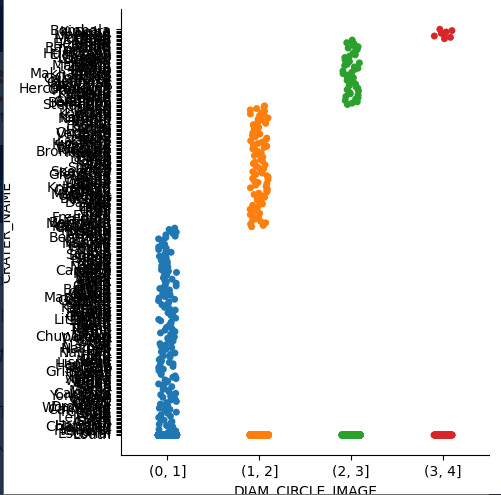
En este caso se relacionan dos varaibles categoricas por lo tanto se utiliza el método catplot
plot5=seaborn.catplot(x='DIAM_CIRCLE_IMAGE', y = 'CRATER_NAME', data=Sub1_DIAM_CIRCLE_IMAGE) plot5.plt.title ('Diametro del crater') plot5.plt.xlabel('Crater') plot5.plt.ylabel('Diametro en mm')
Los resultados:
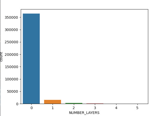
La toma de datos del diámetro del Cráter se realizó hasta 4 capaz de cada, en la siguiente imagen se denota que la mayoría (más de 35000 observaciones) no tiene capaz lo que hace que el detalle de la imagen e información sea menor respecto a las que tienen 3 capaz (alrededor de 1000 observaciones).
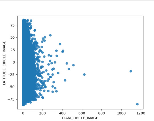
Ahora bien, la relación de la latitud respecto al diámetro registrado del Cráter, el cual esta hasta en 200 km se concentra principalmente en las latitudes de - 75 a - 25, mientras que el cráter de mayor tamaño se ubica en - 75 °. En ese sentido se puede establecer interrogantes cómo ¿Sucedió algún evento geológico que implico la concentración de Cráter en estas latitudes ?, ¿El planeta marte tuvo choques con asteroides en la latitud de -75 que generaran un crater de casi 1200 km ?
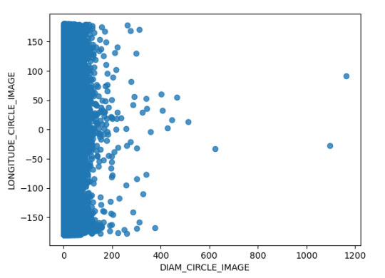
Así mimo, en el análisis se hizo el análisis mediante la siguiente grafica de la dispersión del Diámetro del Cráter y la ubicación longitudinal del mismo; encontrando que el Cráter de mayo tamaño se ubica en 100 y la mayor concentración de longitudinal esta en entorno de la longitud 0. A continuación, presentó la grafica obtenida
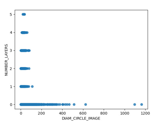
Finalmente se analizaron la relación de dos variables cuantitativas como lo son el diámetro y la cantidad de capaz de los cráteres, en donde identifica que existen observaciones de hasta 5 capaz que no se evidenciaron en grafica anterior, posiblemente por el método de regplot de Pandas es más adecuado para evidenciar el detalle de la dispersión de los datos.
Otro par de variables cuantitativas relacionadas corresponde al diámetro respecto al nombre del Cráter, no obstante como se evidencia a continuación, por la cantidad de datos no es posible identificar fácilmente el nombre del cráter.
0 notes
Photo

Thank you for the tag @naelu - a REALLY ADORABLE BEAN!! This is the simblr vs sims tag created by @catplot! All my sims r cuter than me I cryyy.
rules (C + P from @catplot) make a 3x3 grid for you and your lovely sims, you can either use one of the templates here or make your own from scratch
if you’re not comfortable showing a picture of yourself, feel free to make/use your simself ! (it’s all about the positivity my guy)
I TAG: @nahsims @crytacoo @ridgeport @mousysims and basically everyone bc ur all cute and I wanna see ur cute faces!!! ❤️✨❤️✨
44 notes
·
View notes
Photo

HAPPY HOLIDAYS!!
Hey guys !!! I just wanted to do a little smt smt for y’all (I know it’s like just a doodle (of either u/icon/oc) but I wanted to do smt ?? I can’t make cc / have time to make a grand ol edit so aksdjhf) to show how thankful I am for everyone I’ve met + how I appreciate you guys sm for being super supportive + loving. I didn’t have much time cause I’m going on vacation ( still need to pack haha) + I won’t have access to my game/laptop during the holidays so today was the only free time I had asdjfh. If I had more time, I would have drawn all of you guys buT know that i love each and every one of you because you have made a positive impact in my life and I’m super grateful to have y’all. You matter so much to me and I wish I could give everyone a good ol hug!!! ily + please take care !!
But here’s some ol cheesy ass stuff below (drawings are from l -> r):
@grapfruit :: hONESTLY i dont even need to say anything cause you know how much i love you okay?!?! idk why you stuck w/ me for so long like i’m not even that good of a friend?? like ur super social butterfly + im like a slow fucker at replying but u still stuck w/ me umMM?? legit the v first time u msged me about being from HK i legit fangirled b/c i loved ur sims + style sm and you’re one of the v first frds on here that i really clicked?? like it’s rare for me (even IRL) for me to find ppl im fine w/ but ilysm and i love how we’re super chill tgt + have v similar interests (i mEAN food is #1 priority lets be honest) but I only wish you the best w/ everything in life + i legit care about u sm that i practically adopted u as my sister ok yeah hopefully i can find time to meet up w/ u buT for now ily than ks
@ridgeport :: !!!! margarITA IS2G you’re the best at everything: cc making, story telling, editing okAY you’re the perfect package + i want to thank you for taking the time in doing this + being such a huge part of the community??? i legit can’t imagine this community w/o u?? so thank you for being here + blessing us every day. i hOPE you have a great life cause you deserve everything ok ilysm please have a safe holiday !!!
@chocolat-souffle :: okAY I LOVE HOW WE CLICK SM + we can rant about shit + be open about it + we relate to each other sm?? like our opinions, fashion sense, life in general, food etc?? i’m so thankful that we met on here cause it feels like we would be vvvv good frds if we met irl :’+) ilysm and thNANK YOU again for being so patient w/ me + my slow replies i hope you’re having fun on vacay !!! ilysm okAY
@catplot :: !!!!!! yES U SEE THAT PIXEL THING ON THE CORNER, IT’S OUR FAVOURITE THING AHAHAH bUT I CAN’T BELIEVE THAT WE MAGICALLY FOUND EACH OTHER I S2G IT’S FAITH !!! yOURE 100X BETTER ARTIST THAN ME oKAY and I’m wishing the best okA i hope work isn’t too stressful + youre spending a gol ol jolly time w/ ur loved ones ilysm an d i hope we can continue drawing di!Ck$ tgt for a v long time ily
@meisiu :: i hope you’re doing well w/ ur finals :’+) !! i can’t believe we have sm in common (animal crossing, bujo, sims, canto culture????) like i legit would lOVE to spend more time getting to know you but i just want to rave bout how sweet you are + your builds always amazes me?? i love them sm + once your finals are done, i hope you’ll spend a good time w/ ur loved ones :’+) !! tysm for posting your content everyday !! ily
@whiite-tea :: !!! you’ve been my legit #1 cheerleader since like the beginning. legit you msg me on the daily to make sure + check up if im okay + i’m really thankful for that??! you’re always here supporting me + others + put others first before yourself adsfj yoURE TOO KIND LOVE OKAY?1 remember youre loved + i hope school’s not too stressful :+( !! ilysm !!
@1tens :: yEAH OKAY JES LIKE ILY?? I WANT TO GET TO KNOW U BETTER BUT I KNOW WE’LL BE COOL FRIENDS CAUSE UR SO SWEET + I LOVE UR STYLE SM ??! LIKE U MAKE THE CUTESTS SIMS EVER + UR STYLE + EDITS ARE TO DIE FOR!!!! and you take the time out of your day to comment on like everyone’s post + you’re adorbs okay? im only wishing you the best + tysm for supporting love ilYSM :’+)))
@twikkii :: i drew nissi if you’re okay w/ that :’+) !! but i s2g you’re the cutest ever and my heart is always thinking about you okay?! you make the cutest edits + gameplay pics ever i legit get so excited whenever you post. you’re so sweet + kinda to others & i’m always wishing that you’re doing okay !! ilysm + i’m so thankful i met you- you really taught me things + i appreciate you sm kjadhf have a good holiday love :’+)
@dnasz :: okay honestly everything you post is so cute + aesthetically pleasing?! your builds are amazing (like wanna teach me lOL??! i legit jaw dropped when u post ur most recent ones) + you’re super sweet + kind to others. everyday i look forward in seeing you post cause i know it’ll be amazing :’+) i hope you’ll have a great holiday love !!!
@simsao :: the fact that you match colours so well is inspiring. I’ve always struggled w/ colours + your posts are so unique that it has challenged me to step from my comfort zone + try to explore + play around w/ it more?! so thank you sm for posting + i love your aliens uGH!! your edits are super unique like idk how else to describe them but i love them sm. + your self sim ones atm are my fav omg we legit have sm in common akjsdhf bUT thank you sm for posting + i hope you have a great holiday :’+)
@smubuh :: ABBY!!! okAY i’ve raved about you before but you’re such a sweetheart and a person I really do aspire. You’re kind, hardworking and have a beautiful mind + soul. I rarely look up to anyone but I can safely say you’re one of them !! Thank you for bringing so much to the community - you’ve taught us so much (esp when you have a super busy schedule). I hope you have a great holiday w/ your loved ones + your family :”+) ily !!!
@4fig :: !! i hope you’re doing well w/ ur exams love !! i know i’ve told you so many times but you’re one of the few reasons why i joined this community - your edits are legit my aesthetic ?! every time you post i’m always in aw because you create the most beautiful sims + your editing style is one of my favs. i honestly would love to get to know you better once you’re done w/ everything but you’re really kind + sweet + i only wish you the very best :’+) have a great holiday love !!
@faeflowr :: yeah your edits are my fav okYA?! scratch that EVERYTHING you post is beautiful :’+) your sims, gameplay, edits - they’re all amazing + I love them sm. bUT most importantly you’re so pretty iRl omg?! if i had to choose who’s my fav simblr posts are itll be you cause i love everything you do + your aesthetic is legit exactly what i love aksjdhf ily !! i hope you have a great holiday :+)
@ughplumb :: yEAH ILL FOREVER CALL U UNFPLUMB CAUSE YOU’RE FKING BEAUTIUL I SWEAR U CAN BE A MODEL OK idk why you aren’t like ?? i love how you make ur sims cause i can never make good sims like yours - they’re all beautiful just like you ;’+) aND im excited for you to post but take your time okay ?!? tysm for being here + ily !!! i hope you have a great holiday !!
@mooon-sims :: yeah who do i go to when i need a lookbook?? your styles the best ? i love your new editing style + im so glad youre still here :’+) i know it gets tough esp w/ collage apps + school but im so proud of you okay?1 you’re a strong fighter + im glad you still pull through in posting !!! ily + remember to keep doing you okay?! have a great holiday love :’+)
@blarffy :: !!! okAY YEAH EVERYTHING YOU DO IS PERFECTION AND LIKE EVERY1 CAN BACK ME UP HECK U HAVE LIKE 128736 SPOUCES LINING UP OUTSIDE THE CHAPEL RN bUT thank you sm for posting ?! i know we dont talk that often but youre super sweet (maybe it’s a canadian thing?!? LOOL jokES) but i would love to get to know you better cause youre fking bomb?! thank you for blessing us w/ ur content + i hope you have a great holiday :’+)
@pink-tea :: okAY I MISS YOU AND YOUR POSTS !!! i swear youre so sweet + i love your aesthetic so much ajksdhf buT youre still here always supporting me despite having a super busy life so i thank you for that !! i’m always here supporting you + waiting till you post cause i miss them sm :’+((( i hope youre doing well regardless + remember i always love u !! have a great holiday love!!
@liltofu :: !!! i love lov elove your aesthetic + sims + style so much?! every time you post i get really excited cause you never disappoint? i’m always so jealous of your editing style cause it’s legit my fav thing ever alskdfj + i use like 99% of your recolours cause u pick out the best things to recolour?! bUT i hope youre doing well !! ily + have a great holiday love :’+)
@dust-bubbles :: awh man you’re always here spreading love + i swear youre my lil sunshine :’+) thank you for taking the time out of your day for sendin me love?! like i always smile when you do + i appreciate your unconditional support sm !! i’m wishing you the very best in life cause you deserve it ?! ily + i hope you have a wonderful holiday :’+)
@nolan-sims :: i just want to say thank you so much for the ongoing love + support you give + show to the community. not only are you super sweet + caring but you take the time out of your day in making cc for us?! so thank you for being part of this community - i really appreciate you sm + i only wish good things happen to you + everyone around you :’+) ily + i hope you have a great holiday w/ ur loved ones !!
@ayoshi :: okAY you’re the sweetest little bean ever + your fashion sense is amazing okay ?! i have ALL your cc downloaded so thank you sm for being part of this community + blessing us w/ ur bomb ass cc + edits :’+) i appreciate sm the time + dedication you take out of your day to make stuff for us !! im only wishing you good things + i hope you’ll have a great holiday !!
@obi-uhie :: i WISH I COULD ROCK YOUR CONFIDENCE OKAY ?! you legit inspire me sm + i love how unique your sims are okAY?! keep doing you + i love everything you do :’+) i hope youre having a great holiday love !!
@suspiciouslypinklady :: !! youre so sweet + i love your confidence?! i’m super thankful for the love + support you always give whenever things get tough + i appreciate it sm. it makes things a lot easier + you’re seriously such an angel. i hope you have a great holiday w/ ur loved ones b/c u deserve the v best !!
@viiavi :: okay i just want to say thank you sm for the love + support you give whenever shit hits the fan LOL your kind words + msgs really help me a lot whenver things aren’t the best so I thank you for that. thank you for being so kind, thoughtful + caring to everyone in this community :’+) i really appreciate that sm + i hope you keep doing that !! i hope you have a great holiday !!
@dicoatl :: i swear youre always so kind to others ?! im so sorry you’ve been getting so much negativity these days but i know you’re a super strong person who’s doing their very best + im super proud of you okay!! ive been loving your new edits recently + it really shows youre experimenting a lot + it looks amazing :’+) so thank you for being here okay? have a great holiday !!!
@oakglow :: catherine !! your editing + story telling is amazing?! i mean i can’t write for shit LOL but i love it whenver your post esp knowing you’re busy w/ life. so thank you for that :’+) i hope you + your loved ones a great holiday !!
@simmerjade :: jADE I MISS YOU !!! I HOPE YOU’RE DOING WELL !! you’re one of the v first friends i made here in this community + ik youre super busy rn w/ life but im so glad we’ve met ?! i hope life’s treating you v well + youre not too stressed out from school - i know you can do it :’+) im always here supporting you whatever you do + remember ilysm !!! have a great holiday love !!
@waffle-pxels :: i know we dont talk that often but the times we do youre so kind ?! tysm for being here + supporting me :’+) i really appreciate u sm + i hope youre doing well !! have a great holiday love !!
@simharaa :: i MISS YOU SM OKAY aND I S2G I HOPE YOURE OKAY !! again my heart goes out to you + your family but please take care okay?! you’ve been here since day 1 + i’m super glad we’ve met cause the times we’ve talked i truely treasured sm :’+) i’m loving your edits + im so glad youre back posting again !! i hope you + ur fam a speedy recovery + remember ily !! youre a strong bean !!
@simsluname :: lunA!!! your gifs are amazing + i love how we grew tgt in this community ?? i remember we both started off together + been supporting each other since the v beginning when we joined this community :’+) thank you for being here + blessing us w/ ur gameplay pics + teaching us how to gif ?? like w/o you i wouldn’t have learned ajksdfh so thank you for that & ilysm you’re so cute !!! have a great holiday love !!
@alternacorn-sims :: you’ve been a long time supporter and i’m super thankful for you?! you’re always here liking my stuff + sending positive vibes + love :’+) i hope youre doing well !! please keep doing you + remember that i appreciate you sm :’+) tysm for being here + i hope you have a great holiday w/ ur loved ones!!
@expressgo :: thank you for being so patient w/ me ?!! i’m a super slow replier but we manage to be able to talk + i’m so glad we do?! thank you for reaching out to me at the beginning + i really enjoy talking to you:’+) youre super sweet + we can talk about like everything ?? your cats are adobs + i wish you the best + happy holidays :’+) ily !!
@hazelios :: i seriously have all your cc downloaded in my folder + i appreciate it sm whenever you post content + cc for the community :’+) so thank you for that !! you’re always super kind + sweet whenever we talk and i only wish you the very best !! ily + i hope you have a great holiday !!
@simsthatsparkle :: !!! you’ve been like one of my og supporters for a v long time and i’m super thankful for you being here?! i can’t imagine the love + support i get + idk how else to express my appreciation asjkdfh i only hope you the best + ily !! i hope you have a wonderful holiday love :’+)
@femmesim :: okay you’re a hUGE inspiration to everyone in this community + i’m so thankful that youre here?! your edits + story telling is breath taking + it hits me all the time when you post ?! so thank you sm for creating bomb ass content + telling stories that aren’t often told. please keep doing you!!! i hope you have a great holiday :’+)
#my art#gift for my family#nonsims#queue#o#g#aksjdhf again sorry i couldnt get everyone !! i really wish i could :+(#know that i love you okay?! and i really do mean it#hopefully i can post when im on vacation buT idk kajsdf#so here's smt !!!!#idk im bad at showing my love kajsdhf uagdhfgjla#i wasnt feeling the best yesterday but i want to cheer some of yall up?!
465 notes
·
View notes
Text
..
Tagged by @catplot @mellocakes
name: Cynthia
nickname: Nne, Cent, Uche, Cyn, Cynth
gender: Female
star sign: Aries
height: 5′9
sexuality: Straight
hogwarts house: What’s a hogwarts? ..lol I took a test and I think I was Ravenclaw?
dream trip: Don’t have one
average sleep: 6-8
why i made my tumblr: I don’t know lol .. it was back in 2013 I can’t even remember how I found out about simblr
dog or cat person: DOG
when i made my blog: June 2013
followers: 7471
i tag @everyone :)
29 notes
·
View notes
Text
Week 2 Assignment (Data Analysis Tools)
Week 2 Assignment (Data Analysis Tools) Summary:
The Chi-Square Test for the association between Female Employment Rate and Income Per Person from the GapMinder dataset shows a X2=22.45 and p<.05 indicating an association between the variables.
To make these quantitative variables categorical, femaleemployrate was split into responses of Low (<=50%) and High (>50%) and incomeperperson was split into 3 explanatory groups of Low (<=$1K), Medium ($1K to 10K) and High (>$10K).
The High income group had 65% of countries in the High employment group, while the Medium income group only had 24%. The highest income group had 52.5% of its countries in the High employment group. A post hoc test was needed to determine which groups were different from each other.
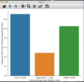
Because 3 comparisons need to be made, the null hypothesis can only be rejected when p<.017. This was the case when comparing the Low or High income groups to the Medium group, which the graph shows as having much lower Female Employment Rates. But there was not a significant difference between the Low and High income groups.
This curious result suggests that while there is an association between the variables, there is likely another unexplored variable that could be responsible for the association.
Crosstab tables from the Python console are listed below, followed by the Python script used:
incomegroup 1Low <=$1K 2Med $1K to <=$10K 3High >$10K
ferhilo
1Low <=50% 18 56 19
2High >50 34 18 21
Percentages for columns in above crosstab table
incomegroup 1Low <=$1K 2Med $1K to <=$10K 3High >$10K
ferhilo
1Low <=50% 0.346154 0.756757 0.475000
2High >50 0.653846 0.243243 0.525000
chi-square value, p value, expected counts
(22.452875462906395, 1.3317418320055155e-05, 2, array([[29.13253012, 41.45783133, 22.40963855],
[22.86746988, 32.54216867, 17.59036145]]))
/opt/anaconda3/lib/python3.8/site-packages/seaborn/categorical.py:3704: UserWarning: The `factorplot` function has been renamed to `catplot`. The original name will be removed in a future release. Please update your code. Note that the default `kind` in `factorplot` (`'point'`) has changed `'strip'` in `catplot`.
warnings.warn(msg)
Compare Low to Med
COMP1v2 1.000000 2.000000
fhilo
0 18 56
1 34 18
COMP1v2 1.000000 2.000000
fhilo
0 0.346154 0.756757
1 0.653846 0.243243
chi-square value, p value, expected counts
(19.582655325443792, 9.633984733934315e-06, 1, array([[30.53968254, 43.46031746],
[21.46031746, 30.53968254]]))
Compare Low to High
COMP1v3 1.000000 3.000000
fhilo
0 18 19
1 34 21
COMP1v3 1.000000 3.000000
fhilo
0 0.346154 0.475000
1 0.653846 0.525000
chi-square value, p value, expected counts
(1.0711888111888124, 0.3006770758566416, 1, array([[20.91304348, 16.08695652],
[31.08695652, 23.91304348]]))
Compare Med to High
COMP2v3 2.000000 3.000000
fhilo
0 56 19
1 18 21
COMP2v3 2.000000 3.000000
fhilo
0 0.756757 0.475000
1 0.243243 0.525000
chi-square value, p value, expected counts
(7.949307692307691, 0.00481057753497139, 1, array([[48.68421053, 26.31578947],
[25.31578947, 13.68421053]]))
Python code:
import numpy
import pandas
#import statsmodels.formula.api as smf
#import statsmodels.stats.multicomp as multi
import scipy.stats
import seaborn
import matplotlib.pyplot as plt
# use set_option to for pandas to show all columns and rows in DataFrame
pandas.set_option('display.max_columns', None)
pandas.set_option('display.max_rows', None)
# bug fix for display formats to avoid run time errors
pandas.set_option('display.float_format', lambda x:'%f'%x)
# other set pandas options here
pandas.set_option('display.max_colwidth',50)
pandas.set_option('display.width', None)
pandas.set_option('display.float_format', lambda x:'%f'%x)
# get dataset from csv in local python folder
data = pandas.read_csv('gapminder_copy.csv', low_memory=(False))
# set variables to numeric and remove errors caused by nulls for 3 variables
data['femaleemployrate'] = pandas.to_numeric(data['femaleemployrate'], errors='coerce')
data['employrate'] = pandas.to_numeric(data['employrate'], errors='coerce')
data['incomeperperson'] = pandas.to_numeric(data['incomeperperson'], errors='coerce')
# Make a subset of the data that removes the entire row if any of the 3 variables are missing data
sub1=data[(data['femaleemployrate']>0) & (data['employrate']>0) & (data['incomeperperson']>0)]
# make a copy of my new subset of the data
sub2 = sub1.copy()
# customized income ranges for further study
sub2['incomegroup'] = pandas.cut(sub2.incomeperperson, [0, 1000, 10000, 100000],labels=["1Low <=$1K", "2Med $1K to <=$10K", "3High >$10K"])
# customized income ranges for further study
sub2['ferhilo'] = pandas.cut(sub2.femaleemployrate, [0, 50, 100],labels=["1Low <=50%", "2High >50"])
# contingency table of observed counts
ct1=pandas.crosstab(sub2['ferhilo'], sub2['incomegroup'])
print (ct1)
print ('')
# column percentages
print ('Percentages for columns in above crosstab table')
colsum=ct1.sum(axis=0)
colpct=ct1/colsum
print(colpct)
print ('')
# chi-square
print ('chi-square value, p value, expected counts')
cs1= scipy.stats.chi2_contingency(ct1)
print (cs1)
# recode to 0/1 and set as numeric for graphing
recode1 = {"1Low <=50%": 0, "2High >50": 1}
sub2['fhilo']= sub2['ferhilo'].map(recode1)
sub2['fhilo'] = pandas.to_numeric(sub2['fhilo'], errors='coerce')
# graph percent with high fememployrate within each income group
seaborn.factorplot(x="incomegroup", y="fhilo", data=sub2, kind="bar", ci=None)
plt.xlabel('Income Group: Low, Medium, High')
plt.ylabel('Proportion with >50% Female Employment Rate')
# perform post hoc comparisons within income groups
# compare Low inc to Med inc groups
recode2 = {"1Low <=$1K" : 1, "2Med $1K to <=$10K": 2}
sub2['COMP1v2']= sub2['incomegroup'].map(recode2)
# contingency table of observed counts
print ('Compare Low to Med')
ct2=pandas.crosstab(sub2['fhilo'], sub2['COMP1v2'])
print (ct2)
# column percentages
colsum=ct2.sum(axis=0)
colpct=ct2/colsum
print(colpct)
print ('chi-square value, p value, expected counts')
cs2= scipy.stats.chi2_contingency(ct2)
print (cs2)
# compare Low inc to High inc
recode3 = {"1Low <=$1K": 1, "3High >$10K": 3}
sub2['COMP1v3']= sub2['incomegroup'].map(recode3)
print('Compare Low to High')
# contingency table of observed counts
ct3=pandas.crosstab(sub2['fhilo'], sub2['COMP1v3'])
print (ct3)
# column percentages
colsum=ct3.sum(axis=0)
colpct=ct3/colsum
print(colpct)
print ('chi-square value, p value, expected counts')
cs3= scipy.stats.chi2_contingency(ct3)
print (cs3)
# compare Med inc to High inc
recode4 = {"2Med $1K to <=$10K": 2, "3High >$10K": 3}
sub2['COMP2v3']= sub2['incomegroup'].map(recode4)
print ('Compare Med to High')
# contingency table of observed counts
ct4=pandas.crosstab(sub2['fhilo'], sub2['COMP2v3'])
print (ct4)
# column percentages
colsum=ct4.sum(axis=0)
colpct=ct4/colsum
print(colpct)
print ('chi-square value, p value, expected counts')
cs4= scipy.stats.chi2_contingency(ct4)
print (cs4)
0 notes
Text
Data Analysis Tools. Module 2: chi square test of independence
Result:
Null hypothesis that there is no difference in the mean of the quantitative variable “femaleemployrate “ across groups for “incomeperperson”
The explantory variable is the income per person in 5 levels (poor, low class, midle class, upper class, rich) and the respond variable is the Female employ rate considering 2 levels ( between 0% and 40% and between 40% and 100%)
distribution for income per person splits into 6 groups and creating a new variable income as categorical variable
poor 80
low class 46
midle class 39
upper class 22
rich 3
NaN 23
Name: income, dtype: int64
distribution for femaleemployrate splits into 2 groups (employ rate between 0% & 40% =0, 40% & 100%=1) and creating a new variable Femaleemploy as categorical variable
0 52
1 126
NaN 35
Name: Femaleemploy, dtype: int64
table of observed counts
income poor low class midle class upper class
Femaleemploy
0 18 14 14 1
1 56 25 18 20
table of observed counts in %
income poor low class midle class upper class
Femaleemploy
0 0.243243 0.358974 0.437500 0.047619
1 0.756757 0.641026 0.562500 0.952381
chi-square value, p value, expected counts
(11.181092289173819, 0.010785880920040842, 3, array([[20.95180723, 11.04216867, 9.06024096, 5.94578313],
[53.04819277, 27.95783133, 22.93975904, 15.05421687]]))
income poor low class midle class upper class
Femaleemploy
0 18 14 14 1
1 56 25 18 20
C:\ProgramData\Anaconda3\lib\site-packages\seaborn\categorical.py:3717: UserWarning: The `factorplot` function has been renamed to `catplot`. The original name will be removed in a future release. Please update your code. Note that the default `kind` in `factorplot` (`'point'`) has changed `'strip'` in `catplot`.
warnings.warn(msg)
Out[42]: Text(6.799999999999997, 0.5, 'Female employ rate')
runfile('G:/QMM/01 Productos/02 USS/04 USS5/python/prueba6-bis.py', wdir='G:/QMM/01 Productos/02 USS/04 USS5/python')
Null hypothesis that there is no difference in the mean of the quantitative variable “femaleemployrate “ across groups for “incomeperperson”
The explantory variable is the income per person in 5 levels (poor, low class, midle class, upper class, rich) and the respond variable is the Female employ rate considering 2 levels ( between 0% and 40% and between 40% and 100%)
distribution for income per person splits into 6 groups and creating a new variable income as categorical variable
poor 54
low class 26
midle class 46
upper class 39
rich 22
NaN 26
Name: income, dtype: int64
distribution for femaleemployrate splits into 2 groups (employ rate between 0% & 40% =0, 40% & 100%=1) and creating a new variable Femaleemploy as categorical variable
0 52
1 126
NaN 35
Name: Femaleemploy, dtype: int64
table of observed counts
income poor low class midle class upper class rich
Femaleemploy
0 11 7 14 14 1
1 41 15 25 18 20
table of observed counts in %
income poor low class midle class upper class rich
Femaleemploy
0 0.211538 0.318182 0.358974 0.437500 0.047619
1 0.788462 0.681818 0.641026 0.562500 0.952381
chi-square value, p value, expected counts
(12.047322395704303, 0.01700281130675494, 4, array([[14.72289157, 6.22891566, 11.04216867, 9.06024096, 5.94578313],
[37.27710843, 15.77108434, 27.95783133, 22.93975904, 15.05421687]]))
income poor low class midle class upper class rich
Femaleemploy
0 11 7 14 14 1
1 41 15 25 18 20
Group poor-low class
table of observed counts
income2 low class poor
Femaleemploy
0 7 11
1 15 41
table of observed counts in %
income2 low class poor
Femaleemploy
0 0.318182 0.211538
1 0.681818 0.788462
chi-square value, p value, expected counts
(0.4636422605172603, 0.49592665933844127, 1, array([[ 5.35135135, 12.64864865],
[16.64864865, 39.35135135]]))
Group poor-midle class
table of observed counts
income3 midle class poor
Femaleemploy
0 14 11
1 25 41
table of observed counts in %
income3 midle class poor
Femaleemploy
0 0.358974 0.211538
1 0.641026 0.788462
chi-square value, p value, expected counts
(1.7476136363636368, 0.18617701296552153, 1, array([[10.71428571, 14.28571429],
[28.28571429, 37.71428571]]))
Group poor-upper class
table of observed counts
income4 poor upper class
Femaleemploy
0 11 14
1 41 18
table of observed counts in %
income4 poor upper class
Femaleemploy
0 0.211538 0.437500
1 0.788462 0.562500
chi-square value, p value, expected counts
(3.8179204693611464, 0.05070713462718701, 1, array([[15.47619048, 9.52380952],
[36.52380952, 22.47619048]]))
Group poor- rich
table of observed counts
income5 poor rich
Femaleemploy
0 11 1
1 41 20
table of observed counts in %
income5 poor rich
Femaleemploy
0 0.211538 0.047619
1 0.788462 0.952381
chi-square value, p value, expected counts
(1.8544659745991714, 0.17326486722177523, 1, array([[ 8.54794521, 3.45205479],
[43.45205479, 17.54794521]]))
Group low class-midle class
table of observed counts
income6 low class midle class
Femaleemploy
0 7 14
1 15 25
table of observed counts in %
income6 low class midle class
Femaleemploy
0 0.318182 0.358974
1 0.681818 0.641026
chi-square value, p value, expected counts
(0.001713911088911098, 0.9669774837195514, 1, array([[ 7.57377049, 13.42622951],
[14.42622951, 25.57377049]]))
Group low class-upper class
table of observed counts
income7 low class upper class
Femaleemploy
0 7 14
1 15 18
table of observed counts in %
income7 low class upper class
Femaleemploy
0 0.318182 0.437500
1 0.681818 0.562500
chi-square value, p value, expected counts
(0.3596148170011807, 0.5487202341134262, 1, array([[ 8.55555556, 12.44444444],
[13.44444444, 19.55555556]]))
Group low class-rich
table of observed counts
income8 low class rich
Femaleemploy
0 7 1
1 15 20
table of observed counts in %
income8 low class rich
Femaleemploy
0 0.318182 0.047619
1 0.681818 0.952381
chi-square value, p value, expected counts
(3.5608128478664187, 0.059158762972845974, 1, array([[ 4.09302326, 3.90697674],
[17.90697674, 17.09302326]]))
Group midle class-upperclass
table of observed counts
income9 midle class upper class
Femaleemploy
0 14 14
1 25 18
table of observed counts in %
income9 midle class upper class
Femaleemploy
0 0.358974 0.437500
1 0.641026 0.562500
chi-square value, p value, expected counts
(0.1845768844769572, 0.667469088625999, 1, array([[15.38028169, 12.61971831],
[23.61971831, 19.38028169]]))
Group midle class-rich
table of observed counts
income10 midle class rich
Femaleemploy
0 14 1
1 25 20
table of observed counts in %
income10 midle class rich
Femaleemploy
0 0.358974 0.047619
1 0.641026 0.952381
chi-square value, p value, expected counts
(5.4945054945054945, 0.01907632210177841, 1, array([[ 9.75, 5.25],
[29.25, 15.75]]))
Group upper class-rich
table of observed counts
income11 rich upper class
Femaleemploy
0 1 14
1 20 18
table of observed counts in %
income11 rich upper class
Femaleemploy
0 0.047619 0.437500
1 0.952381 0.562500
chi-square value, p value, expected counts
(7.673854558270678, 0.005602664662587936, 1, array([[ 5.94339623, 9.05660377],
[15.05660377, 22.94339623]]))
0 notes
Text
Party affiliation vs Obama ratings by age groups
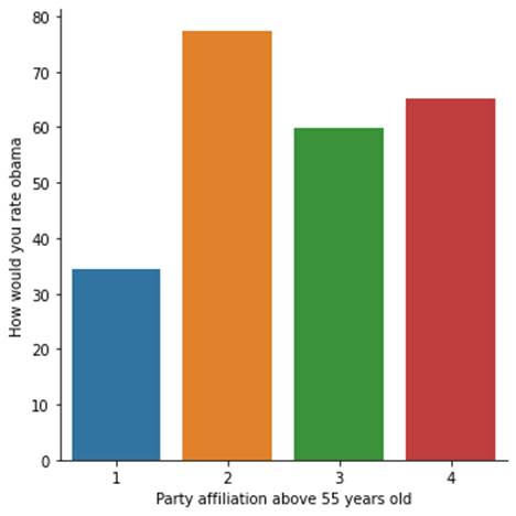
In this study, I would like to use run an ANOVA correlation coefficient to find out if party affiliation is associated with Obama ratings, and then use two age groups as moderator – between 18 and 54 years old, and 55 years or older.
Results:
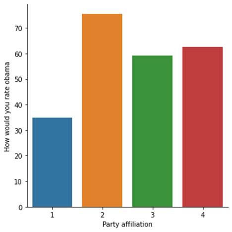
Without the moderator, the Prob score is 3.90e-116 and F-statistics is 219.2, indicating a strong correlation.
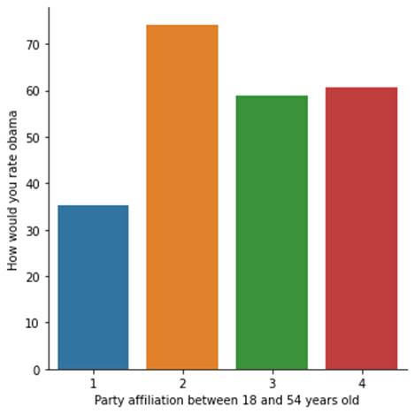
With age as moderator, we see similar association in distributions among the two age groups, although older people who have no party affiliations rated Obama higher.
Code
# -*- coding: utf-8 -*-
"""
Created on Mon Sep 21 10:18:43 2015
@author: jml
"""
# ANOVA
import numpy
import pandas
import statsmodels.formula.api as smf
import statsmodels.stats.multicomp as multi
import seaborn
import matplotlib.pyplot as plt
data = pandas.read_csv('ool_pds.csv', low_memory=False)
# party affiliation
# 1:Republican, 2:Democrat, 3:Independent, 4:Other, -1:Refused
data['W1_C1'] = pandas.to_numeric(data['W1_C1'], errors='coerce')
# [Barack Obama] How would you rate
data['W1_D1'] = pandas.to_numeric(data['W1_D1'], errors='coerce')
# PPAGECAT: Age - 7 Categories
data['PPAGECAT'] = pandas.to_numeric(data['PPAGECAT'], errors='coerce')
sub1 = data[(data['W1_C1']>=1) & (data['W1_C1']<=4) & (data['W1_D1']>=1) & (data['W1_D1']<=99) & (data['PPAGECAT']>=1) & (data['PPAGECAT']<=7)]
model1 = smf.ols(formula='W1_D1 ~ C(W1_C1)', data=sub1).fit()
print (model1.summary())
print ("means for Party affiliations")
m1= sub1.groupby('W1_C1').mean()
print (m1)
print ("standard deviation for mean Party affiliations")
st1= sub1.groupby('W1_C1').std()
print (st1)
# bivariate bar graph
seaborn.factorplot(x="W1_C1", y="W1_D1", data=sub1, kind="bar", ci=None)
plt.xlabel('Party affiliation')
plt.ylabel('How would you rate obama')
sub2=sub1[(sub1['PPAGECAT']>=1) & (sub1['PPAGECAT']<=4)] #54 or younger
sub3=sub1[(sub1['PPAGECAT']>=5) & (sub1['PPAGECAT']<=7)] #55 or older
print ('association between party affiliation and Obama ratings for those who are between 18 and 54 years old')
model2 = smf.ols(formula='W1_D1 ~ C(W1_C1)', data=sub2).fit()
print (model2.summary())
print ('association between party affiliation and Obama ratings for those who are above 54 years old')
model3 = smf.ols(formula='W1_D1 ~ C(W1_C1)', data=sub3).fit()
print (model3.summary())
print ("means for party affiliation vs Obama ratings for those who are between 18 and 54 years old")
m3= sub2.groupby('W1_C1').mean()
print (m3)
print ("Means for party affiliation vs Obama ratings for those who are above 54 years old")
m4 = sub3.groupby('W1_C1').mean()
print (m4)
seaborn.factorplot(x="W1_C1", y="W1_D1", data=sub2, kind="bar", ci=None)
plt.xlabel('Party affiliation between 18 and 54 years old')
plt.ylabel('How would you rate obama')
seaborn.factorplot(x="W1_C1", y="W1_D1", data=sub3, kind="bar", ci=None)
plt.xlabel('Party affiliation above 55 years old')
plt.ylabel('How would you rate obama')
Results
OLS Regression Results
==============================================================================
Dep. Variable: W1_D1 R-squared: 0.325
Model: OLS Adj. R-squared: 0.323
Method: Least Squares F-statistic: 219.2
Date: Mon, 16 Nov 2020 Prob (F-statistic): 3.90e-116
Time: 09:46:27 Log-Likelihood: -6074.1
No. Observations: 1373 AIC: 1.216e+04
Df Residuals: 1369 BIC: 1.218e+04
Df Model: 3
Covariance Type: nonrobust
=================================================================================
coef std err t P>|t| [0.025 0.975]
---------------------------------------------------------------------------------
Intercept 34.8985 1.440 24.229 0.000 32.073 37.724
C(W1_C1)[T.2] 40.6217 1.632 24.890 0.000 37.420 43.823
C(W1_C1)[T.3] 24.2801 1.746 13.908 0.000 20.855 27.705
C(W1_C1)[T.4] 27.6822 2.944 9.403 0.000 21.907 33.457
==============================================================================
Omnibus: 99.662 Durbin-Watson: 2.005
Prob(Omnibus): 0.000 Jarque-Bera (JB): 122.244
Skew: -0.672 Prob(JB): 2.85e-27
Kurtosis: 3.573 Cond. No. 7.28
==============================================================================
Warnings:
[1] Standard Errors assume that the covariance matrix of the errors is correctly specified.
means for Party affiliations
CASEID W1_CASEID W1_WEIGHT1 ... PPT612 PPWORK PPNET
W1_C1 ...
1 1074.822335 1119.304569 1.966889 ... 0.218274 2.862944 0.822335
2 1179.302594 1228.017291 0.872340 ... 0.182997 2.995677 0.783862
3 1137.830952 1185.430952 1.278669 ... 0.209524 2.840476 0.811905
4 1129.532258 1176.419355 1.086908 ... 0.241935 2.806452 0.790323
[4 rows x 240 columns]
standard deviation for mean Party affiliations
CASEID W1_CASEID W1_WEIGHT1 ... PPT612 PPWORK PPNET
W1_C1 ...
1 660.456702 691.693381 1.542526 ... 0.578590 2.203082 0.383204
2 636.686082 666.974779 1.245637 ... 0.483135 2.151877 0.411907
3 680.088596 712.417932 1.464464 ... 0.581254 2.098023 0.391254
4 687.015826 718.273466 1.435755 ... 0.533638 2.164079 0.410402
[4 rows x 240 columns]
association between party affiliation and Obama ratings for those who are between 18 and 54 years old
OLS Regression Results
==============================================================================
Dep. Variable: W1_D1 R-squared: 0.298
Model: OLS Adj. R-squared: 0.296
Method: Least Squares F-statistic: 116.4
Date: Mon, 16 Nov 2020 Prob (F-statistic): 8.08e-63
Time: 09:46:27 Log-Likelihood: -3663.3
No. Observations: 825 AIC: 7335.
Df Residuals: 821 BIC: 7353.
Df Model: 3
Covariance Type: nonrobust
=================================================================================
coef std err t P>|t| [0.025 0.975]
---------------------------------------------------------------------------------
Intercept 35.1736 1.870 18.809 0.000 31.503 38.844
C(W1_C1)[T.2] 38.9499 2.136 18.234 0.000 34.757 43.143
C(W1_C1)[T.3] 23.6124 2.249 10.498 0.000 19.198 28.027
C(W1_C1)[T.4] 25.4653 3.905 6.521 0.000 17.800 33.131
==============================================================================
Omnibus: 44.959 Durbin-Watson: 1.920
Prob(Omnibus): 0.000 Jarque-Bera (JB): 50.940
Skew: -0.586 Prob(JB): 8.68e-12
Kurtosis: 3.327 Cond. No. 7.24
==============================================================================
Warnings:
[1] Standard Errors assume that the covariance matrix of the errors is correctly specified.
association between party affiliation and Obama ratings for those who are above 54 years old
OLS Regression Results
==============================================================================
Dep. Variable: W1_D1 R-squared: 0.363
Model: OLS Adj. R-squared: 0.360
Method: Least Squares F-statistic: 103.4
Date: Mon, 16 Nov 2020 Prob (F-statistic): 5.47e-53
Time: 09:46:27 Log-Likelihood: -2407.3
No. Observations: 548 AIC: 4823.
Df Residuals: 544 BIC: 4840.
Df Model: 3
Covariance Type: nonrobust
=================================================================================
coef std err t P>|t| [0.025 0.975]
---------------------------------------------------------------------------------
Intercept 34.4605 2.253 15.297 0.000 30.035 38.886
C(W1_C1)[T.2] 42.9267 2.525 17.003 0.000 37.968 47.886
C(W1_C1)[T.3] 25.4321 2.768 9.187 0.000 19.994 30.870
C(W1_C1)[T.4] 30.8087 4.462 6.905 0.000 22.044 39.574
==============================================================================
Omnibus: 62.487 Durbin-Watson: 1.938
Prob(Omnibus): 0.000 Jarque-Bera (JB): 86.729
Skew: -0.821 Prob(JB): 1.47e-19
Kurtosis: 4.051 Cond. No. 7.37
==============================================================================
Warnings:
[1] Standard Errors assume that the covariance matrix of the errors is correctly specified.
means for party affiliation vs Obama ratings for those who are between 18 and 54 years old
C:\Apps\Anaconda3\lib\site-packages\seaborn\categorical.py:3666: UserWarning: The `factorplot` function has been renamed to `catplot`. The original name will be removed in a future release. Please update your code. Note that the default `kind` in `factorplot` (`'point'`) has changed `'strip'` in `catplot`.
warnings.warn(msg)
CASEID W1_CASEID W1_WEIGHT1 ... PPT612 PPWORK PPNET
W1_C1 ...
1 1092.471074 1137.933884 2.339593 ... 0.338843 2.247934 0.876033
2 1188.581864 1238.060453 0.930930 ... 0.274559 2.458438 0.808564
3 1168.154982 1217.387454 1.399492 ... 0.317343 2.424354 0.841328
4 1080.194444 1124.583333 1.318103 ... 0.388889 2.805556 0.833333
[4 rows x 240 columns]
Means for party affiliation vs Obama ratings for those who are above 54 years old
CASEID W1_CASEID W1_WEIGHT1 ... PPT612 PPWORK PPNET
W1_C1 ...
1 1046.723684 1089.644737 1.373505 ... 0.026316 3.842105 0.736842
2 1166.898990 1214.592593 0.794022 ... 0.060606 3.713805 0.750842
3 1082.677852 1127.308725 1.058917 ... 0.013423 3.597315 0.758389
4 1197.846154 1248.192308 0.766792 ... 0.038462 2.807692 0.730769
0 notes
Note
What was your old name
hey anon !! my old name was catturday-sim, i changed it to catplot because it was way too long for me and i didn’t like the -sim part !! #:^)
11 notes
·
View notes
Text
Data Tools Week 4
For this assignment, I placed the summary up front and the added the code with out output after to simplify the reading due to the amount of code used. I am using the Gap Minder data set. The explanatory variable is incomeperperson and the response variable is lifeepextancy.
For this assignment, the moderator variable is set as urbanrate.
For all of the tests, the data was grouped based on income. Group 1=low income ; Group 2=medium income ; Group 3=middle income ; Group 4=high income.
Data management tasks included converting values to numeric, making blank entries NAN, dropping NAN, and creating functions to group data according to urban rate, income per person, and life expectancy.
For the ANOVA Test, I needed to create a categorical variable for the initial test. I generated 4 categorical groups using the incomeperperson qualitative variable by creating a new function. Once the intial ANOVA was run, I created the moderator variable using urbanrate and created 4 sub groups for urban rates. I then ran the ANOVA Test against the original subgroup and the new urban rate group
The ANOVA was run and shows that there is no statistical significance, P-Values greater than .05, with groups 1,2, and 4-in relationship to the explanatory and response variables with the moderator variable. Group 3 has a significant P Value when comparing urbanrate against incomeperperson and lifeexpectancy. So ANOVA shows that group 3's explanatory and response variables have a relationship with the moderator variable.
For the Chi Test I created 2 categorical variables from incomeperperson and lifeexpectancy from the dataset. Then the Chi Test was run against these 2 variables. Next I generated the moderator variable using urbanrate. Once urbanrate was broken into 4 groups, I ran the Chi Test with the original variables and the each new subgroup for urbanrate.
The Chi Test's output shows that when the moderator variable is added into the test, Groups 3 & 4 generate a P-Value lower than .05, highlighting a significant relationship with the urbanrate variable. A bar graph also displays that there is a positive relationship trend when the variables are compared and tested.
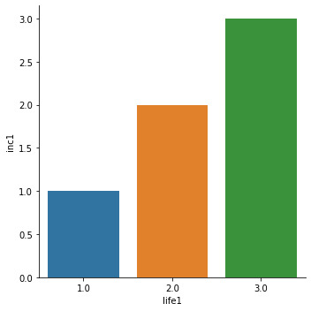
There was minimal data management tasks needed for the last test since the dataset is made up of all quantitative variables. The urbanrate variable was broken into 4 groups and the Pearson test was run against the original dataframe and each new urbanrate subgroup. The Person Correlation test is the final test for this assignment. For this test, the variables remained the same as the previous 2 tests.
The correlation test shows that the group 1 has weak relationships due to the low r-value(.039) and p-value (.08). The other 3 groups generate r-values and p-values that show a strengthening relationship as urban rate and income rate increases. The r-value increases with each group and shows a stronger relationship while the p-value remains below .05 and indicates a significant relationship. The below scatter plot shows the variables plotted and sorted by color. The green and red dots represent groups 3 & 4.
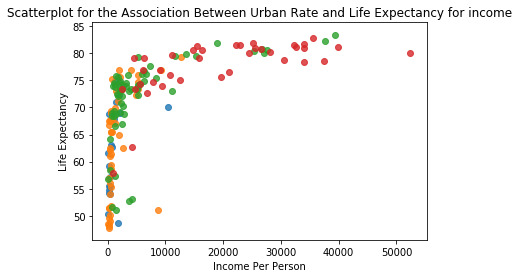
To summarize, each test refined and straightened the hypothesis that urban rate has a relationship with life expectancy and income per person. In the case of ANOVA, I can accept the Alternate Hypothesis that there is a relationship between the variables. The Chi Test continues to support the alternate hypothesis by showing that groups 3 and 4 have a low Outputs ANOVA Outputincome rate levels OLS Regression Results ==============================================================================Dep. Variable: lifeexpectancy R-squared: 0.314Model: OLS Adj. R-squared: 0.306Method: Least Squares F-statistic: 39.67Date: Wed, 09 Sep 2020 Prob (F-statistic): 6.59e-15Time: 10:54:10 Log-Likelihood: -616.44No. Observations: 176 AIC: 1239.Df Residuals: 173 BIC: 1248.Df Model: 2 Covariance Type: nonrobust ================================================================================== coef std err t P>|t| [0.025 0.975]----------------------------------------------------------------------------------Intercept 66.7201 0.695 96.031 0.000 65.349 68.091C(inc1)[T.2.0] 11.7342 1.940 6.047 0.000 7.904 15.564C(inc1)[T.3.0] 14.0902 1.940 7.261 0.000 10.260 17.920==============================================================================Omnibus: 16.013 Durbin-Watson: 1.955Prob(Omnibus): 0.000 Jarque-Bera (JB): 18.340Skew: -0.775 Prob(JB): 0.000104Kurtosis: 2.689 Cond. No. 3.47============================================================================== Warnings:[1] Standard Errors assume that the covariance matrix of the errors is correctly specified.means for Life Expectancy by Income Level lifeexpectancy incomeperperson urbanrateinc1 1.0 66.720147 2351.783373 48.6745592.0 78.454300 15911.876831 75.6450003.0 80.810350 32577.507070 82.352000standard deviation for life expectancy by income level lifeexpectancy incomeperperson urbanrateinc1 1.0 9.082408 2321.563488 20.2330892.0 3.148828 4368.956577 19.8172603.0 1.313176 6725.720440 12.141864urban rate levelsassociation between Life Expectancy and and Income Per Person for Urban Group 1 Low OLS Regression Results ==============================================================================Dep. Variable: lifeexpectancy R-squared: 0.053Model: OLS Adj. R-squared: 0.000Method: Least Squares F-statistic: 1.000Date: Wed, 09 Sep 2020 Prob (F-statistic): 0.331Time: 10:54:10 Log-Likelihood: -69.311No. Observations: 20 AIC: 142.6Df Residuals: 18 BIC: 144.6Df Model: 1 Covariance Type: nonrobust ================================================================================== coef std err t P>|t| [0.025 0.975]----------------------------------------------------------------------------------Intercept 61.7514 1.872 32.985 0.000 57.818 65.685C(inc1)[T.2.0] 8.3726 8.372 1.000 0.331 -9.217 25.962==============================================================================Omnibus: 3.105 Durbin-Watson: 2.341Prob(Omnibus): 0.212 Jarque-Bera (JB): 1.272Skew: 0.100 Prob(JB): 0.529Kurtosis: 1.781 Cond. No. 4.60============================================================================== Warnings:[1] Standard Errors assume that the covariance matrix of the errors is correctly specified.association between Life Expectancy and and Income Per Person for Urban Group 2 Medium OLS Regression Results ==============================================================================Dep. Variable: lifeexpectancy R-squared: 0.053Model: OLS Adj. R-squared: 0.034Method: Least Squares F-statistic: 2.785Date: Wed, 09 Sep 2020 Prob (F-statistic): 0.101Time: 10:54:11 Log-Likelihood: -190.40No. Observations: 52 AIC: 384.8Df Residuals: 50 BIC: 388.7Df Model: 1 Covariance Type: nonrobust ================================================================================== coef std err t P>|t| [0.025 0.975]----------------------------------------------------------------------------------Intercept 63.1583 1.345 46.966 0.000 60.457 65.859C(inc1)[T.2.0] 16.1827 9.697 1.669 0.101 -3.295 35.660==============================================================================Omnibus: 15.846 Durbin-Watson: 1.985Prob(Omnibus): 0.000 Jarque-Bera (JB): 3.826Skew: -0.224 Prob(JB): 0.148Kurtosis: 1.749 Cond. No. 7.28============================================================================== Warnings:[1] Standard Errors assume that the covariance matrix of the errors is correctly specified.association between Life Expectancy and and Income Per Person for Urban Group 3 Middle OLS Regression Results ==============================================================================Dep. Variable: lifeexpectancy R-squared: 0.258Model: OLS Adj. R-squared: 0.235Method: Least Squares F-statistic: 10.98Date: Wed, 09 Sep 2020 Prob (F-statistic): 8.12e-05Time: 10:54:11 Log-Likelihood: -214.90No. Observations: 66 AIC: 435.8Df Residuals: 63 BIC: 442.4Df Model: 2 Covariance Type: nonrobust ================================================================================== coef std err t P>|t| [0.025 0.975]----------------------------------------------------------------------------------Intercept 70.4463 0.875 80.551 0.000 68.699 72.194C(inc1)[T.2.0] 8.1936 2.766 2.963 0.004 2.667 13.720C(inc1)[T.3.0] 10.8094 2.766 3.909 0.000 5.283 16.336==============================================================================Omnibus: 29.947 Durbin-Watson: 2.301Prob(Omnibus): 0.000 Jarque-Bera (JB): 49.457Skew: -1.731 Prob(JB): 1.82e-11Kurtosis: 5.448 Cond. No. 3.73============================================================================== Warnings:[1] Standard Errors assume that the covariance matrix of the errors is correctly specified.association between Life Expectancy and and Income Per Person for Urban Group 4 High OLS Regression Results ==============================================================================Dep. Variable: lifeexpectancy R-squared: 0.053Model: OLS Adj. R-squared: 0.000Method: Least Squares F-statistic: 1.000Date: Wed, 09 Sep 2020 Prob (F-statistic): 0.331Time: 10:54:11 Log-Likelihood: -69.311No. Observations: 20 AIC: 142.6Df Residuals: 18 BIC: 144.6Df Model: 1 Covariance Type: nonrobust ================================================================================== coef std err t P>|t| [0.025 0.975]----------------------------------------------------------------------------------Intercept 61.7514 1.872 32.985 0.000 57.818 65.685C(inc1)[T.2.0] 8.3726 8.372 1.000 0.331 -9.217 25.962==============================================================================Omnibus: 3.105 Durbin-Watson: 2.341Prob(Omnibus): 0.212 Jarque-Bera (JB): 1.272Skew: 0.100 Prob(JB): 0.529Kurtosis: 1.781 Cond. No. 4.60============================================================================== Warnings:[1] Standard Errors assume that the covariance matrix of the errors is correctly specified.means for Life Expectancy by Income Per Person for Urban Group 1 lifeexpectancy incomeperperson urbanrate inc1urb1 1.0 62.17 1304.690529 18.679 1.05means for Life Expectancy by Income Per Person for Urban Group 2 lifeexpectancy incomeperperson urbanrate inc1urb1 2.0 63.469481 1764.840618 37.084615 1.019231means for Life Expectancy by Income Per Person for Urban Group 3 lifeexpectancy incomeperperson urbanrate inc1urb1 3.0 72.173803 6497.448498 63.328485 1.272727means for Life Expectancy by Income Per Person for Urban Group 4 lifeexpectancy incomeperperson urbanrate inc1urb1 4.0 77.682868 19550.870875 86.79 2.052632 Chi Test OutputStandard Deviation for Life Expectancycount 191.000000mean 69.753524std 9.708621min 47.79400025% 64.44700050% 73.13100075% 76.593000max 83.394000Name: lifeexpectancy, dtype: float64Standard Deviation for Income Per Personcount 190.000000mean 8740.966076std 14262.809083min 103.77585725% 748.24515150% 2553.49605675% 9379.891165max 105147.437697Name: incomeperperson, dtype: float64Chi Square Analysis for Explanatory and Response VariablesC:\Users\sockm\anaconda3\lib\site-packages\seaborn\categorical.py:3669: UserWarning: The `factorplot` function has been renamed to `catplot`. The original name will be removed in a future release. Please update your code. Note that the default `kind` in `factorplot` (`'point'`) has changed `'strip'` in `catplot`. warnings.warn(msg)inc1 1.0 2.0 3.0life1 1.0 136 0 02.0 0 20 03.0 0 0 20inc1 1.0 2.0 3.0life1 1.0 1.0 0.0 0.02.0 0.0 1.0 0.03.0 0.0 0.0 1.0chi-square value, p value, expected counts(351.99999999999994, 6.488502127788041e-75, 4, array([[105.09090909, 15.45454545, 15.45454545], [ 15.45454545, 2.27272727, 2.27272727], [ 15.45454545, 2.27272727, 2.27272727]]))Adding Moderator Variableinc1 1.0 2.0life1 1.0 19 02.0 0 1inc1 1.0 2.0 3.0life1 1.0 0.139706 0.00 NaN2.0 0.000000 0.05 NaNchi-square value, p value, expected counts(4.487534626038781, 0.03414288228006565, 1, array([[18.05, 0.95], [ 0.95, 0.05]]))inc1 1.0 2.0life1 1.0 51 02.0 0 1inc1 1.0 2.0 3.0life1 1.0 0.375 0.00 NaN2.0 0.000 0.05 NaNchi-square value, p value, expected counts(12.49519415609381, 0.00040800022640174056, 1, array([[5.00192308e+01, 9.80769231e-01], [9.80769231e-01, 1.92307692e-02]]))inc1 1.0 2.0 3.0life1 1.0 54 0 02.0 0 6 03.0 0 0 6inc1 1.0 2.0 3.0life1 1.0 0.397059 0.0 0.02.0 0.000000 0.3 0.03.0 0.000000 0.0 0.3chi-square value, p value, expected counts(132.00000000000003, 1.4542497475734214e-27, 4, array([[44.18181818, 4.90909091, 4.90909091], [ 4.90909091, 0.54545455, 0.54545455], [ 4.90909091, 0.54545455, 0.54545455]]))inc1 1.0 2.0 3.0life1 1.0 12 0 02.0 0 12 03.0 0 0 14inc1 1.0 2.0 3.0life1 1.0 0.088235 0.0 0.02.0 0.000000 0.6 0.03.0 0.000000 0.0 0.7chi-square value, p value, expected counts(76.0, 1.2242617888987312e-15, 4, array([[3.78947368, 3.78947368, 4.42105263], [3.78947368, 3.78947368, 4.42105263], [4.42105263, 4.42105263, 5.15789474]])) Pearson Correlation Output urban rate levelsassociation between urbanrate and life expecatany for LOW income countries(0.39070589367158226, 0.08852079337577021) association between urbanrate and life expecatany for Medium income countries(0.4750165695713443, 0.0004908618152919306) association between urbanrate and life expecatany for Middle income countries(0.5530182478009116, 2.600193675208846e-06) association between urbanrate and life expecatany for High income countries(0.6062786995430565, 5.474886254266103e-05) AxesSubplot(0.125,0.125;0.775x0.755)AxesSubplot(0.125,0.125;0.775x0.755)AxesSubplot(0.125,0.125;0.775x0.755)AxesSubplot(0.125,0.125;0.775x0.755) ANOVA Code# ANOVA import numpy as npimport pandas as pdimport statsmodels.formula.api as smfimport statsmodels.stats.multicomp as multiimport seabornimport matplotlib.pyplot as plt data = pd.read_csv('gapminder.csv', low_memory=False) #Convert Blank to NAN and numeric conversiondata['incomeperperson']=data.incomeperperson.replace(" " ,np.nan)data['incomeperperson'] = pd.to_numeric(data.incomeperperson) data['lifeexpectancy']=data.lifeexpectancy.replace(" " ,np.nan)data['lifeexpectancy'] = pd.to_numeric(data.lifeexpectancy) data['urbanrate'] = data.urbanrate.replace(" ",np.nan)data['urbanrate'] = pd.to_numeric(data.urbanrate) # subset variables in new data frame, sub1sub1=data[['lifeexpectancy', 'incomeperperson', 'urbanrate']].dropna() #assign variables to sub4 #Standard Deviationsprint ("standard deviation for life expectancy by income level")st1= data['lifeexpectancy'].std()print (st1) ## Income Levelsdef INCOMERATE(row): if row['incomeperperson'] < 10000: return 1 if row['incomeperperson'] >10000 and row['incomeperperson'] <=25000: return 2 if row['incomeperperson'] >25000 and row['incomeperperson'] <=100000: return 3 if row['incomeperperson'] >100000: return 4 #incomerate function appliedprint ("income rate levels")sub2=sub1sub2['inc1'] = INCOMERATEsub2['inc1'] = data.apply (lambda row: INCOMERATE (row),axis=1) #b = sub2['inc1'].head (n=50)#print(b) #Initial ANOVA with Means and STD DEV model1 = smf.ols(formula='lifeexpectancy ~ C(inc1)', data=sub2).fit()print (model1.summary()) print ("means for Life Expectancy by Income Level")m1= sub2.groupby('inc1').mean()print (m1) print ("standard deviation for life expectancy by income level")st1= sub2.groupby('inc1').std()print (st1) ## Urban Rate Levelsdef URBANRATE(row): if row['urbanrate'] < 25: return 1 if row['urbanrate'] >25 and row['urbanrate'] <=50: return 2 if row['urbanrate'] >50 and row['urbanrate'] <=75: return 3 if row['urbanrate'] >75: return 4 print ("urban rate levels")sub2=sub1sub2['urb1'] = URBANRATEsub2['urb1'] = data.apply (lambda row: URBANRATE (row),axis=1) ##Moderator Levelssub3=sub2[(sub2['urb1']== 1)]sub4=sub2[(sub2['urb1']== 2)]sub5=sub2[(sub2['urb1']== 3)]sub6=sub2[(sub2['urb1']== 4)] #Moderation ANOVA URB1print ('association between Life Expectancy and and Income Per Person for Urban Group 1')model2 = smf.ols(formula='lifeexpectancy ~ C(inc1)', data=sub3).fit()print (model2.summary()) print ('association between Life Expectancy and and Income Per Person for Urban Group 2')model3 = smf.ols(formula='lifeexpectancy ~ C(inc1)', data=sub4).fit()print (model3.summary()) print ('association between Life Expectancy and and Income Per Person for Urban Group 3')model4 = smf.ols(formula='lifeexpectancy ~ C(inc1)', data=sub5).fit()print (model4.summary()) print ('association between Life Expectancy and and Income Per Person for Urban Group 4')model5 = smf.ols(formula='lifeexpectancy ~ C(inc1)', data=sub3).fit()print (model5.summary()) ## Meansprint ("means for Life Expectancy by Income Per Person for Urban Group 1")m1= sub3.groupby('urb1').mean()print (m1) print ("means for Life Expectancy by Income Per Person for Urban Group 2")m2= sub4.groupby('urb1').mean()print (m2) print ("means for Life Expectancy by Income Per Person for Urban Group 3")m3= sub5.groupby('urb1').mean()print (m3) print ("means for Life Expectancy by Income Per Person for Urban Group 4")m4= sub6.groupby('urb1').mean()print (m4)## End ANOVA Chi Test Code# Chi Square import numpy as npimport pandas as pdimport statsmodels.formula.api as smfimport statsmodels.stats.multicomp as multiimport seaborn as sbimport matplotlib.pyplot as pltimport scipy.stats as stats data = pd.read_csv('gapminder.csv', low_memory=False) #Convert Blank to NAN and numeric conversiondata['incomeperperson']=data.incomeperperson.replace(" " ,np.nan)data['incomeperperson'] = pd.to_numeric(data.incomeperperson) data['lifeexpectancy']=data.lifeexpectancy.replace(" " ,np.nan)data['lifeexpectancy'] = pd.to_numeric(data.lifeexpectancy) data['urbanrate'] = data.urbanrate.replace(" ",np.nan)data['urbanrate'] = pd.to_numeric(data.urbanrate) #Standard deviationsprint("Standard Deviation for Life Expectancy")dev1=data.lifeexpectancy.describe()print(dev1) print("Standard Deviation for Income Per Person")dev2=data.incomeperperson.describe()print(dev2) # subset variables in new data frame, sub1sub1=data[['lifeexpectancy', 'incomeperperson', 'urbanrate']].dropna() #assign variables to sub4 ## Income Levelsdef INCOMERATE(row): if row['incomeperperson'] < 10000: return 1 if row['incomeperperson'] >10000 and row['incomeperperson'] <=25000: return 2 if row['incomeperperson'] >25000 and row['incomeperperson'] <=100000: return 3 if row['incomeperperson'] >100000: return 4 #incomerate function applied#print ("income rate levels")sub2=sub1sub2['inc1'] = INCOMERATEsub2['inc1'] = data.apply (lambda row: INCOMERATE (row),axis=1) #Life Expectancy Levelsdef LIFEEXPECT(row): if row['lifeexpectancy'] < 55: return 1 if row['lifeexpectancy'] >55 and row['incomeperperson'] <=65: return 2 if row['lifeexpectancy'] >65 and row['incomeperperson'] <=75: return 3 if row['lifeexpectancy'] >75: return 4 #life expectancy function appliedsub2=sub1sub2['life1'] = INCOMERATEsub2['life1'] = data.apply (lambda row: INCOMERATE (row),axis=1) #Initial Chi Square with Means and STD DEVprint("Chi Square Analysis for Explanatory and Response Variables") # Bar Graph plot for first bivariatessb.factorplot(x="life1", y="inc1", data=sub2, kind="bar", ci=None)plt.xlabel=("Life Expectancy Rate")plt.ylabel=("Income Rate") # chi-square for first two variable# contingency table of observed countsct1=pd.crosstab(sub2['life1'], sub2['inc1'])print (ct1) # column percentagescolsum=ct1.sum(axis=0)colpct=ct1/colsumprint(colpct) # chi-squareprint ('chi-square value, p value, expected counts')cs1= stats.chi2_contingency(ct1)print (cs1) # Moderator areaprint("Adding Moderator Variable")## Urban Rate Levelsdef URBANRATE(row): if row['urbanrate'] < 25: return 1 if row['urbanrate'] >25 and row['urbanrate'] <=50: return 2 if row['urbanrate'] >50 and row['urbanrate'] <=75: return 3 if row['urbanrate'] >75: return 4 # URBANRATE Applied#print ("urban rate levels")sub2=sub1sub2['urb1'] = URBANRATEsub2['urb1'] = data.apply (lambda row: URBANRATE (row),axis=1) ##Urban Group Levelssub3=sub2[(sub2['urb1']== 1)]sub4=sub2[(sub2['urb1']== 2)]sub5=sub2[(sub2['urb1']== 3)]sub6=sub2[(sub2['urb1']== 4)] # chi-square with moderator variable added#Moderator Group 1# contingency table of observed countsct2=pd.crosstab(sub3['life1'], sub3['inc1'])print (ct2) # column percentagescolsum2=ct2.sum(axis=0)colpct2=ct2/colsumprint(colpct2) # chi-squareprint ('chi-square value, p value, expected counts')cs2= stats.chi2_contingency(ct2)print (cs2) #Moderator Group 2# contingency table of observed countsct3=pd.crosstab(sub4['life1'], sub4['inc1'])print (ct3) # column percentagescolsum3=ct3.sum(axis=0)colpct3=ct3/colsumprint(colpct3) # chi-squareprint ('chi-square value, p value, expected counts')cs3= stats.chi2_contingency(ct3)print (cs3) #Moderator Group 3# contingency table of observed countsct4=pd.crosstab(sub5['life1'], sub5['inc1'])print (ct4) # column percentagescolsum4=ct4.sum(axis=0)colpct4=ct4/colsumprint(colpct4) # chi-squareprint ('chi-square value, p value, expected counts')cs4= stats.chi2_contingency(ct4)print (cs4) #Moderator Group 4# contingency table of observed countsct5=pd.crosstab(sub6['life1'], sub6['inc1'])print (ct5) # column percentagescolsum5=ct5.sum(axis=0)colpct5=ct5/colsumprint(colpct5) # chi-squareprint ('chi-square value, p value, expected counts')cs5= stats.chi2_contingency(ct5)print (cs5)##End CHI Test Pearson Code @author: sockm"""import pandas as pdimport numpy as npimport seaborn as sbimport scipy.statsimport matplotlib.pyplot as plt gmdata = pd.read_csv('gapminder.csv', low_memory=False) #Convert Blank to NAN and numeric conversiongmdata['urbanrate']=gmdata.urbanrate.replace(" " ,np.nan)gmdata['urbanrate'] = pd.to_numeric(gmdata.urbanrate) gmdata['incomeperperson']=gmdata.incomeperperson.replace(" " ,np.nan)gmdata['incomeperperson'] = pd.to_numeric(gmdata.incomeperperson) gmdata['lifeexpectancy']=gmdata.incomeperperson.replace(" " ,np.nan)gmdata['lifeexpectancy'] = pd.to_numeric(gmdata.incomeperperson) sub1=gmdata[['incomeperperson', 'urbanrate','lifeexpectancy']].dropna()print(sub1) #Scatter Plotsb.regplot(x='incomeperperson', y='lifeexpectancy', fit_reg=False, data=sub1)plt.xlabel("Income Per Person")plt.ylabel("Life Expectancy")#plt.title('Scatterplot for the Association Between Urban Rate and Income Per Person Rate') ## Pearon for first 2 variablesprint ('association between life expectancy and income per person')print (scipy.stats.pearsonr(sub1['lifeexpectancy'], sub1['incomeperperson'])) ##Exp & Resp Variable groupings## Income Levelssub2=sub1 ##Moderdate Variable## Urban Rate Levels to Categoricaldef URBANRATE(row): if row['urbanrate'] < 25: return 1 if row['urbanrate'] >26 and row['urbanrate'] <49: return 2 if row['urbanrate'] >50 and row['urbanrate'] < 74: return 3 if row['urbanrate'] >75: return 4 #urbanrate function appliedprint ("urban rate levels")sub2['urb1'] = URBANRATEsub2['urb1'] = sub1.apply (lambda row: URBANRATE (row),axis=1) #sub3=sub2[['inc1', 'life1', 'urb1']].head (n=50)#print(sub3) sub3=sub2[(sub2['urb1']== 1)]sub4=sub2[(sub2['urb1']== 2)]sub5=sub2[(sub2['urb1']== 3)]sub6=sub2[(sub2['urb1']== 4)] print ('association between urbanrate and life expecatany for LOW income countries')print (scipy.stats.pearsonr(sub3['urbanrate'], sub3['lifeexpectancy']))print (' ')print ('association between urbanrate and life expecatany for Medium income countries')print (scipy.stats.pearsonr(sub4['urbanrate'], sub4['lifeexpectancy']))print (' ')print ('association between urbanrate and life expecatany for Middle income countries')print (scipy.stats.pearsonr(sub5['urbanrate'], sub5['lifeexpectancy']))print (' ')print ('association between urbanrate and life expecatany for High income countries')print (scipy.stats.pearsonr(sub6['urbanrate'], sub6['lifeexpectancy']))print (' ') ## Scatter Plots#%%scat1 = sb.regplot(x='urb1', y='lifeexpectancy', fit_reg=False,data=sub3)plt.xlabel("Urban Rate")plt.ylabel("Life Expectancy")plt.title('Scatterplot for the Association Between Urban Rate and Life Expectancy for LOW income countries')print (scat1)#%%scat2 = sb.regplot(x='urb1', y='lifeexpectancy', fit_reg=False, data=sub4)plt.xlabel("Urban Rate")plt.ylabel("Life Expectancy")plt.title('Scatterplot for the Association Between Urban Rate and Life Expectancy for MIDDLE income countries')print (scat2)#%%scat3 = sb.regplot(x='urb1', y='lifeexpectancy',fit_reg=False, data=sub5)plt.xlabel("Urban Rate")plt.ylabel("Life Expectancy")plt.title('Scatterplot for the Association Between Urban Rate and Life Expectancy for MEDIUM income countries')print (scat3)#%%scat4 = sb.regplot(x='urb1', y='lifeexpectancy',fit_reg=False, data=sub6)plt.xlabel("Urban Rate")plt.ylabel("Life Expectancy")plt.title('Scatterplot for the Association Between Urban Rate and Life Expectancy for HIGH income countries')print (scat4)
0 notes
Text
Exploring Statistical Interactions
This assignment aims to statistically assess the evidence, provided by NESARC codebook, in favor of or against the association between alcoholic drinkers and Final weight. More specifically, I examined the statistical interaction between individuals who drank at least 1 alcoholic drink in life (2-level categorical explanatory ,S2AQ1) and Final Weight of individuals (quantitative response variable, WEIGHT (measured in Weighting factor)), moderated by variable “SOCPDX12”(Categorical), which indicates people having social phobia in the last 12 months. This effect is characterized statistically as an interaction, which is a third variable that affects the direction and/or the strength of the relationship between the explanatory and the response variable and help us understand the moderation. Since I have a categorical explanatory variable (Individuals who drank at least 1 alcoholic drink in life) and a quantitative response variable (Final Weight), I ran ANOVA (Analysis of Variance) test to examine the patterns of the association between them (C->Q),by directly measuring the F-statistic value and the p-value. In addition, in order visualize graphically this association, I used catplot function (seaborn library) to produce a bivariate graph. Furthermore, I took 2-level categorical variable, therefore, I did not perform the post hoc test, using Tukey hsd approach.
Regarding the third variable, I examined if individuals having social phobia in the last 12 months, moderates the significant association between individuals who drank at least 1 alcoholic drink in life and Final Weight of individuals. Put it another way, are individuals who drank at least 1 alcoholic drink in life related to Final Weight of individuals for each level of moderating variable (0=No and 1=Yes), that is for individuals who did not have social phobia in last 12 months and for individuals who had? Therefore, I set new data frames (sub2 and sub3) that include either individuals who fell into each category (Yes or No) and ran the Analysis of Variance(ANOVA) for each subgroup separately, measuring both the F-statistics and the p-values. Finally, with catplot function (seaborn library) I created two bivariate bar graphs, one for each level of the moderating variable, in order to visualize the differences and the effect of the moderator upon the statistical relationship between individuals who drank at least 1 alcoholic drink in life and Final Weight of individuals. For the code and the output I used Jupyter notebook (IDE).
The moderating variable that I used for the statistical interaction is:

PROGRAM:
import pandas as pd import numpy as np import statsmodels.formula.api as smf import seaborn import matplotlib.pyplot as plt data = pd.read_csv('nesarc_pds.csv',low_memory=False)
subsetc1 = data.copy()
subsetc1['S2AQ1'] = pd.to_numeric(subsetc1['S2AQ1'],errors='coerce') subsetc1['WEIGHT'] = pd.to_numeric(subsetc1['WEIGHT'],errors='coerce')
sub1 = subsetc1[['S2AQ1','WEIGHT']].dropna()
model1 = smf.ols(formula='WEIGHT ~ C(S2AQ1)',data=sub1).fit() print(model1.summary())
print('means') m1 = sub1.groupby('S2AQ1').mean() print(m1) print('Standard Deviation') m2 = sub1.groupby('S2AQ1').std() print(m2)
seaborn.catplot(x="S2AQ1", y="WEIGHT", data=sub1, kind="bar", ci=None) plt.xlabel('Drank at least 1 alcoholic drink in life') plt.ylabel('Final Weight')
data['S2AQ5A'] = pd.to_numeric(data['SOCPDX12'],errors='coerce') subsetc2 = data[(data['SOCPDX12']==0)] subsetc3 = data[(data['SOCPDX12']==1)]
sub2 = subsetc2[['S2AQ1','WEIGHT']].dropna() sub3 = subsetc3[['S2AQ1','WEIGHT']].dropna()
model2 = smf.ols(formula='WEIGHT ~ C(S2AQ1)',data=sub2).fit() print(model2.summary())
print('means') m3 = sub2.groupby('S2AQ1').mean() print(m3) print('Standard Deviation') m4 = sub2.groupby('S2AQ1').std() print(m4)
seaborn.catplot(x="S2AQ1", y="WEIGHT", data=sub2, kind="bar", ci=None) plt.xlabel('Drank at least 1 alcoholic drink in life') plt.ylabel('Final Weight')
model3 = smf.ols(formula='WEIGHT ~ C(S2AQ1)',data=sub3).fit() print(model3.summary())
print('means') m5 = sub3.groupby('S2AQ1').mean() print(m5) print('Standard Deviation') m6 = sub3.groupby('S2AQ1').std() print(m6)
seaborn.catplot(x="S2AQ1", y="WEIGHT", data=sub3, kind="bar", ci=None) plt.xlabel('Drank at least 1 alcoholic drink in life') plt.ylabel('Final Weight')
OUTPUT:
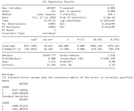
An Analysis of Variance(ANOVA) test revealed that from the NESARC codebook, the individuals who drank at least 1 alcoholic drink in life (2-level categorical explanatory variable) and Final Weight of individuals (quantitative response variable) were significantly associated, F=194.3, 1 df, p=4.52e-44 (where p-value is written in scientific notation).
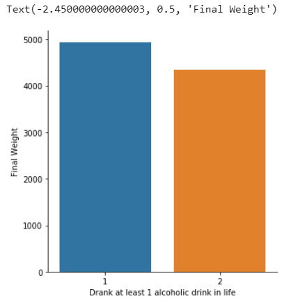
In the bivariate graph (C->Q) presented above, we can see the correlation between individuals who drank at least 1 alcoholic drink in life (explanatory variable) and Final Weight of individuals (response variable). Thus, it is explained in the above graph that individuals who drink alcohol gain more weight than those who don’t drink alcohol.

In the first place, for the moderating variable equal to 0, which is individuals who don’t have social phobia in last 12 months (sub2), a Analysis of Variance(ANOVA) test revealed that among the NESARC codebook, the individuals who drank at least 1 alcoholic drink in life (explanatory variable) and Final Weight of individuals (response variable) were significantly associated, F=200.6,1 df, p=1.99e-45 (where p-value is written in scientific notation). As a result, since the F-statistic value is very large and the p-value is significantly small, we can assume that there is a strong positive relationship between these two variables, when taking into account the subgroup of individuals who did not have social phobia in the last 12 months.

In the bivariate bar graph (C->Q) presented above, we can see the correlation between the individuals who drank at least 1 alcoholic drink in life (explanatory variable) and Final Weight of individuals (response variable), in the subgroup of individuals who did not have social phobia in the last 12 months(sub2). Obviously, it shows a positive relationship between these two variables, which means that the individuals who drank at least 1 alcoholic drink in life directly affects the Final weight of individuals, regarding the individuals who did not have social phobia in the last 12 months.
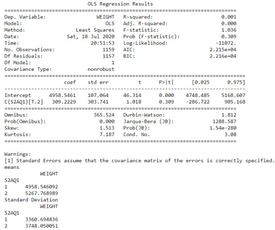
Secondly, for the moderating variable equal to 1, which is those individuals who had social phobia in the last 12 months (sub3), an Analysis of Variance(ANOVA) test revealed that among NESARC codebook, the individuals who drank at least 1 alcoholic drink in life (explanatory variable) and Final Weight of individuals (response variable) were not significantly associated, F=1.036,1 df, p=0.309. As a result, since the F-statistic value is quite small and the p-value is significantly large, we can assume that there is no statistic relationship between these two variables, when taking into account the subgroup of individuals who had social phobia in the last 12 months.

In the bivariate bar graph (C->Q) presented above, we can see the correlation between individuals who drank at least 1 alcoholic drink in life (explanatory variable) and Final Weight of individuals (response variable), in the subgroup of individuals who had social phobia in the last 12 months (sub3). In fact, there is no positive relationship between these two variable, for those who had social phobia in the last 12 months.
SUMMARY:
It seems that both the direction and the size of the relationship between individuals who drank at least 1 alcoholic drink in life and Final Weight of individuals, is heavily affected by social phobia in the last 12 months. In other words, the individuals who had social phobia in the last 12 months, the correlation is considerably weak, whereas who did not have social phobia, the correlation is significantly strong and positive. Thus, the third variable moderates the association between individuals who drank at least 1 alcoholic drink in life and Final Weight of individuals.
0 notes
Text
Assignment_4 Testing a Potential Moderator
Chi-Square Test of Independence
#“libraries”
import pandas import numpy import scipy.stats import seaborn import matplotlib.pyplot as plt
data = pandas.read_csv(‘addhealth_pds.csv’, low_memory=False)
#print ('Converting variables to numeric’)
data['H1SU1’] = pandas.to_numeric(data['H1SU1’], errors='coerce’) data['H1NB6’] = pandas.to_numeric(data['H1NB6’], errors='coerce’)
#print ('Coding missing values’)
data[“H1SU1”] = data[“H1SU1”].replace(6, numpy.nan) data[“H1SU1”] = data[“H1SU1”].replace(9, numpy.nan) data[“H1SU1”] = data[“H1SU1”].replace(8, numpy.nan) data[“H1NB6”] = data[“H1NB6”].replace(6, numpy.nan) data[“H1NB6”] = data[“H1NB6”].replace(8, numpy.nan)
#print ('contingency table of observed counts’)
ct1=pandas.crosstab(data['H1SU1’], data['H1NB6’]) print (ct1)
print ('column percentages’) colsum=ct1.sum(axis=0) colpct=ct1/colsum print(colpct)
#print ('chi-square value, p value, expected counts’) cs1= scipy.stats.chi2_contingency(ct1) print (cs1)
#print ('set variable types’) data[“H1NB6”] = data[“H1NB6”].astype('category’) data['H1SU1’] = pandas.to_numeric(data['H1SU1’], errors='coerce’)
seaborn.factorplot(x=“H1NB6”, y=“H1SU1”, data=data, kind=“bar”, ci=None) plt.xlabel('Happiness Level Living in Neighbourhood 5=Very Happy’) plt.ylabel('Considered Suicide in Past 12 Months’)
recode1= {1: 1, 2: 2} data['COMP1v2’]= data[“H1NB6”].map(recode1)
#print ('contigency table of observed counts’) ct2=pandas.crosstab(data['H1SU1’], data['COMP1v2’]) print (ct2)
#print ('column percentages’) colsum=ct2.sum(axis=0) colpct=ct2/colsum print(colpct)
#print ('chi-square value, p value, expected counts’) cs2= scipy.stats.chi2_contingency(ct2) print (cs2)
recode2= {1: 1, 3: 3} data['COMP1v3’]= data[“H1NB6”].map(recode2)
#print ('contigency table of observed counts’) ct3=pandas.crosstab(data['H1SU1’], data['COMP1v3’]) print (ct3)
#print ('column percentages’) colsum=ct3.sum(axis=0) colpct=ct3/colsum print(colpct)
#print ('chi-square value, p value, expected counts’) cs3= scipy.stats.chi2_contingency(ct3) print (cs3)
recode3= {1: 1, 4: 4} data['COMP1v4’]= data[“H1NB6”].map(recode3)
#print ('contigency table of observed counts’) ct4=pandas.crosstab(data['H1SU1’], data['COMP1v4’]) print (ct4)
print ('column percentages’) colsum=ct4.sum(axis=0) colpct=ct4/colsum print(colpct)
#print ('chi-square value, p value, expected counts’) cs4= scipy.stats.chi2_contingency(ct4) print (cs4)
recode4= {1: 1, 5: 5} data['COMP1v5’]= data[“H1NB6”].map(recode4)
#print ('contigency table of observed counts’) ct5=pandas.crosstab(data['H1SU1’], data['COMP1v5’]) print (ct5)
#print ('column percentages’) colsum=ct5.sum(axis=0) colpct=ct5/colsum print(colpct)
#print ('chi-square value, p value, expected counts’) cs5= scipy.stats.chi2_contingency(ct5) print (cs5)
recode5= {2: 2, 3: 3} data['COMP2v3’]= data[“H1NB6”].map(recode5)
#print ('contigency table of observed counts’) ct6=pandas.crosstab(data['H1SU1’], data['COMP2v3’]) print (ct6)
#print ('column percentages’) colsum=ct6.sum(axis=0) colpct=ct6/colsum print(colpct)
#print ('chi-square value, p value, expected counts’) cs6= scipy.stats.chi2_contingency(ct6) print (cs6)
recode6= {2: 2, 4: 4} data['COMP2v4’]= data[“H1NB6”].map(recode6)
#print ('contigency table of observed counts’) ct7=pandas.crosstab(data['H1SU1’], data['COMP2v4’]) print (ct7)
#print ('column percentages’) colsum=ct7.sum(axis=0) colpct=ct7/colsum print(colpct)
#print ('chi-square value, p value, expected counts’) cs7= scipy.stats.chi2_contingency(ct7) print (cs7)
recode7= {2: 2, 5: 5} data['COMP2v5’]= data[“H1NB6”].map(recode7)
#print ('contigency table of observed counts’) ct8=pandas.crosstab(data['H1SU1’], data['COMP2v5’]) print (ct8)
#print ('column percentages’) colsum=ct8.sum(axis=0) colpct=ct8/colsum print(colpct)
#print ('chi-square value, p value, expected counts’) cs8= scipy.stats.chi2_contingency(ct8) print (cs8)
recode8= {3: 3, 4: 4} data['COMP3v4’]= data[“H1NB6”].map(recode8)
#print ('contigency table of observed counts’) ct9=pandas.crosstab(data['H1SU1’], data['COMP3v4’]) print (ct9)
#print ('column percentages’) colsum=ct9.sum(axis=0) colpct=ct9/colsum print(colpct)
#print ('chi-square value, p value, expected counts’) cs9= scipy.stats.chi2_contingency(ct9) print (cs9)
recode9= {3: 3, 5: 5} data['COMP3v5’]= data[“H1NB6”].map(recode9)
#print ('contigency table of observed counts’) ct10=pandas.crosstab(data['H1SU1’], data['COMP3v5’]) print (ct10)
#print ('column percentages’) colsum=ct10.sum(axis=0) colpct=ct10/colsum print(colpct)
#print ('chi-square value, p value, expected counts’) cs10= scipy.stats.chi2_contingency(ct10) print (cs10)
recode10= {4: 4, 5: 5} data['COMP4v5’]= data[“H1NB6”].map(recode10)
#print ('contigency table of observed counts’) ct11=pandas.crosstab(data['H1SU1’], data['COMP4v5’]) print (ct11)
#print ('column percentages’) colsum=ct11.sum(axis=0) colpct=ct11/colsum print(colpct)
#print ('chi-square value, p value, expected counts’) cs11= scipy.stats.chi2_contingency(ct11) print (cs11)
OUTPUT
Converting variables to numeric Coding missing values contingency table of observed counts H1NB6 1.0 2.0 3.0 4.0 5.0 H1SU1 0.0 138 287 1142 2016 2023 1.0 55 74 227 284 180 column percentages H1NB6 1.0 2.0 3.0 4.0 5.0 H1SU1 0.0 0.715026 0.795014 0.834186 0.876522 0.918293 1.0 0.284974 0.204986 0.165814 0.123478 0.081707 (122.34711107270866, 1.6837131211401846e-25, 4, array([[ 168.37192655, 314.93401805, 1194.30656707, 2006.50482415, 1921.88266418], [ 24.62807345, 46.06598195, 174.69343293, 293.49517585, 281.11733582]])) /Users/tyler2k/anaconda3/lib/python3.7/site-packages/seaborn/categorical.py:3666: UserWarning: The `factorplot` function has been renamed to `catplot`. The original name will be removed in a future release. Please update your code. Note that the default `kind` in `factorplot` (`'point’`) has changed `'strip’` in `catplot`. warnings.warn(msg) COMP1v2 1.0 2.0 H1SU1 0.0 138 287 1.0 55 74 COMP1v2 1.0 2.0 H1SU1 0.0 0.715026 0.795014 1.0 0.284974 0.204986 (4.0678278591878705, 0.04370744446565526, 1, array([[148.05956679, 276.94043321], [ 44.94043321, 84.05956679]])) COMP1v3 1.0 3.0 H1SU1 0.0 138 1142 1.0 55 227 COMP1v3 1.0 3.0 H1SU1 0.0 0.715026 0.834186 1.0 0.284974 0.165814 (15.43912984309443, 8.52056112101083e-05, 1, array([[ 158.15620999, 1121.84379001], [ 34.84379001, 247.15620999]])) COMP1v4 1.0 4.0 H1SU1 0.0 138 2016 1.0 55 284 column percentages COMP1v4 1.0 4.0 H1SU1 0.0 0.715026 0.876522 1.0 0.284974 0.123478 (38.163564128380244, 6.505592851611984e-10, 1, array([[ 166.755716, 1987.244284], [ 26.244284, 312.755716]])) COMP1v5 1.0 5.0 H1SU1 0.0 138 2023 1.0 55 180 COMP1v5 1.0 5.0 H1SU1 0.0 0.715026 0.918293 1.0 0.284974 0.081707 (80.60217876116656, 2.760549400154315e-19, 1, array([[ 174.07053422, 1986.92946578], [ 18.92946578, 216.07053422]])) COMP2v3 2.0 3.0 H1SU1 0.0 287 1142 1.0 74 227 COMP2v3 2.0 3.0 H1SU1 0.0 0.795014 0.834186 1.0 0.204986 0.165814 (2.783546208781313, 0.09523708259004951, 1, array([[ 298.19017341, 1130.80982659], [ 62.80982659, 238.19017341]])) COMP2v4 2.0 4.0 H1SU1 0.0 287 2016 1.0 74 284 COMP2v4 2.0 4.0 H1SU1 0.0 0.795014 0.876522 1.0 0.204986 0.123478 (17.110228714530386, 3.527182890794104e-05, 1, array([[ 312.43254416, 1990.56745584], [ 48.56745584, 309.43254416]])) COMP2v5 2.0 5.0 H1SU1 0.0 287 2023 1.0 74 180 COMP2v5 2.0 5.0 H1SU1 0.0 0.795014 0.918293 1.0 0.204986 0.081707 (51.44490204835613, 7.363494652526882e-13, 1, array([[ 325.23790952, 1984.76209048], [ 35.76209048, 218.23790952]])) COMP3v4 3.0 4.0 H1SU1 0.0 1142 2016 1.0 227 284 COMP3v4 3.0 4.0 H1SU1 0.0 0.834186 0.876522 1.0 0.165814 0.123478 (12.480541372399653, 0.00041121300778005455, 1, array([[1178.33251567, 1979.66748433], [ 190.66748433, 320.33251567]])) COMP3v5 3.0 5.0 H1SU1 0.0 1142 2023 1.0 227 180 COMP3v5 3.0 5.0 H1SU1 0.0 0.834186 0.918293 1.0 0.165814 0.081707 (58.33047436979929, 2.2158497377240775e-14, 1, array([[1213.01371781, 1951.98628219], [ 155.98628219, 251.01371781]])) COMP4v5 4.0 5.0 H1SU1 0.0 2016 2023 1.0 284 180 COMP4v5 4.0 5.0 H1SU1 0.0 0.876522 0.918293 1.0 0.123478 0.081707 (20.793289909858167, 5.116190394045173e-06, 1, array([[2063.00244282, 1975.99755718], [ 236.99755718, 227.00244282]]))
Generating a Correlation Coefficient
Code
import pandas import numpy import seaborn import scipy import matplotlib.pyplot as plt
data = pandas.read_csv(‘addhealth_pds.csv’, low_memory=False)
“converting variables to numeric” data[“H1SU2”] = data[“H1SU2”].convert_objects(convert_numeric=True) data[“H1WP8”] = data[“H1WP8”].convert_objects(convert_numeric=True)
“Coding missing values”
data[“H1SU2”] = data[“H1SU2”].replace(6, numpy.nan) data[“H1SU2”] = data[“H1SU2”].replace(7, numpy.nan) data[“H1SU2”] = data[“H1SU2”].replace(8, numpy.nan)
data[“H1WP8”] = data[“H1WP8”].replace(96, numpy.nan) data[“H1WP8”] = data[“H1WP8”].replace(97, numpy.nan) data[“H1WP8”] = data[“H1WP8”].replace(98, numpy.nan)
scat1 = seaborn.regplot(x='H1SU2’, y='H1WP8’, fit_reg=True, data=data) plt.xlabel('Number of suicide attempts in past 12 months’) plt.ylabel('how many of the past 7 days there was at least one parent in the room with the respondent for their evening meal’) plt.title('Scatterplot for the association between respondents suicide attemps and how many days they ate their evening meal with their parents’)
data_clean=data.dropna()
print ('association between H1SU2 and H1WP8’) print (scipy.stats.pearsonr(data_clean['H1SU2’], data_clean['H1WP8’]))
ANOVA
#post hoc ANOVA
import pandas
import numpy
import statsmodels.formula.api as smf
import statsmodels.stats.multicomp as multi
data = pandas.read_csv(‘addhealth_pds.csv’, low_memory=False)
print(“converting variables to numeric”)
data[“H1SU1”] = data[“H1SU1”].convert_objects(convert_numeric=True)
data[“H1NB5”] = data[“H1NB5”].convert_objects(convert_numeric=True)
data[“H1NB6”] = data[“H1NB6”].convert_objects(convert_numeric=True)
print(“Coding missing values”)
data[“H1SU1”] = data[“H1SU1”].replace(6, numpy.nan)
data[“H1SU1”] = data[“H1SU1”].replace(9, numpy.nan)
data[“H1SU1”] = data[“H1SU1”].replace(8, numpy.nan)
data[“H1NB5”] = data[“H1NB5”].replace(6, numpy.nan)
data[“H1NB6”] = data[“H1NB6”].replace(6, numpy.nan)
data[“H1NB6”] = data[“H1NB6”].replace(8, numpy.nan)
#F-Statistic
model1 = smf.ols(formula=‘H1SU1 ~ C(H1NB6)’, data=data)
results1 = model1.fit()
print (results1.summary())
sub1 = data[['H1SU1’, 'H1NB6’]].dropna()
print ('means for H1SU1 by happiness level in neighbourhood’)
m1= sub1.groupby('H1NB6’).mean()
print (m1)
print ('standard deviation for H1SU1 by happiness level in neighbourhood’)
sd1 = sub1.groupby('H1NB6’).std()
print (sd1)
#more tahn 2 lvls
sub2 = sub1[['H1SU1’, 'H1NB6’]].dropna()
model2 = smf.ols(formula='H1SU1 ~ C(H1NB6)’, data=sub2).fit()
print (model2.summary())
print ('2: means for H1SU1 by happiness level in neighbourhood’)
m2= sub2.groupby('H1NB6’).mean()
print (m2)
print ('2: standard deviation for H1SU1 by happiness level in neighbourhood’)
sd2 = sub2.groupby('H1NB6’).std()
print (sd2)
mc1 = multi.MultiComparison(sub2['H1SU1’], sub2 ['H1NB6’])
res1 = mc1.tukeyhsd()
print(res1.summary())
ANOVA RESULTS
converting variables to numeric
Coding missing values
OLS Regression Results
==============================================================================
Dep. Variable: H1SU1 R-squared: 0.019
Model: OLS Adj. R-squared: 0.018
Method: Least Squares F-statistic: 31.16
Date: Sat, 24 Aug 2019 Prob (F-statistic): 9.79e-26
Time: 17:16:11 Log-Likelihood: -2002.8
No. Observations: 6426 AIC: 4016.
Df Residuals: 6421 BIC: 4049.
Df Model: 4
Covariance Type: nonrobust
===================================================================================
coef std err t P>|t| [0.025 0.975]
———————————————————————————–
Intercept 0.2850 0.024 11.976 0.000 0.238 0.332
C(H1NB6)[T.2.0] -0.0800 0.029 -2.713 0.007 -0.138 -0.022
C(H1NB6)[T.3.0] -0.1192 0.025 -4.688 0.000 -0.169 -0.069
C(H1NB6)[T.4.0] -0.1615 0.025 -6.519 0.000 -0.210 -0.113
C(H1NB6)[T.5.0] -0.2033 0.025 -8.191 0.000 -0.252 -0.155
==============================================================================
Omnibus: 2528.245 Durbin-Watson: 1.952
Prob(Omnibus): 0.000 Jarque-Bera (JB): 7313.190
Skew: 2.173 Prob(JB): 0.00
Kurtosis: 5.903 Cond. No. 15.0
==============================================================================
Warnings:
[1] Standard Errors assume that the covariance matrix of the errors is correctly specified.
means for H1SU1 by happiness level in neighbourhood
H1SU1
H1NB6
1.0 0.284974
2.0 0.204986
3.0 0.165814
4.0 0.123478
5.0 0.081707
standard deviation for H1SU1 by happiness level in neighbourhood
H1SU1
H1NB6
1.0 0.452576
2.0 0.404252
3.0 0.372050
4.0 0.329057
5.0 0.273980
/For all other conversions use the data-type specific converters pd.to_datetime, pd.to_timedelta and pd.to_numeric.
data[“H1SU1”] = data[“H1SU1”].convert_objects(convert_numeric=True)
For all other conversions use the data-type specific converters pd.to_datetime, pd.to_timedelta and pd.to_numeric.
data[“H1NB5”] = data[“H1NB5”].convert_objects(convert_numeric=True)
For all other conversions use the data-type specific converters pd.to_datetime, pd.to_timedelta and pd.to_numeric.
data[“H1NB6”] = data[“H1NB6”].convert_objects(convert_numeric=True)
OLS Regression Results
==============================================================================
Dep. Variable: H1SU1 R-squared: 0.019
Model: OLS Adj. R-squared: 0.018
Method: Least Squares F-statistic: 31.16
Date: Sat, 24 Aug 2019 Prob (F-statistic): 9.79e-26
Time: 17:16:11 Log-Likelihood: -2002.8
No. Observations: 6426 AIC: 4016.
Df Residuals: 6421 BIC: 4049.
Df Model: 4
Covariance Type: nonrobust
===================================================================================
coef std err t P>|t| [0.025 0.975]
———————————————————————————–
Intercept 0.2850 0.024 11.976 0.000 0.238 0.332
C(H1NB6)[T.2.0] -0.0800 0.029 -2.713 0.007 -0.138 -0.022
C(H1NB6)[T.3.0] -0.1192 0.025 -4.688 0.000 -0.169 -0.069
C(H1NB6)[T.4.0] -0.1615 0.025 -6.519 0.000 -0.210 -0.113
C(H1NB6)[T.5.0] -0.2033 0.025 -8.191 0.000 -0.252 -0.155
==============================================================================
Omnibus: 2528.245 Durbin-Watson: 1.952
Prob(Omnibus): 0.000 Jarque-Bera (JB): 7313.190
Skew: 2.173 Prob(JB): 0.00
Kurtosis: 5.903 Cond. No. 15.0
==============================================================================
Warnings:
[1] Standard Errors assume that the covariance matrix of the errors is correctly specified.
2: means for H1SU1 by happiness level in neighbourhood
H1SU1
H1NB6
1.0 0.284974
2.0 0.204986
3.0 0.165814
4.0 0.123478
5.0 0.081707
2: standard deviation for H1SU1 by considered suicide in past 12 months
H1SU1
H1NB6
1.0 0.452576
2.0 0.404252
3.0 0.372050
4.0 0.329057
5.0 0.273980
Multiple Comparison of Means - Tukey HSD,FWER=0.05
=============================================
group1 group2 meandiff lower upper reject
———————————————
1.0 2.0 -0.08 -0.1604 0.0004 False
1.0 3.0 -0.1192 -0.1885 -0.0498 True
1.0 4.0 -0.1615 -0.2291 -0.0939 True
1.0 5.0 -0.2033 -0.271 -0.1356 True
2.0 3.0 -0.0392 -0.0925 0.0142 False
2.0 4.0 -0.0815 -0.1326 -0.0304 True
2.0 5.0 -0.1233 -0.1745 -0.0721 True
3.0 4.0 -0.0423 -0.0731 -0.0115 True
3.0 5.0 -0.0841 -0.1152 -0.0531 True
4.0 5.0 -0.0418 -0.0687 -0.0149 True
0 notes