#UrbanRealities

[utaesthetics]

CTF-UrbanReality

[wondrousnovels]

“To have someone understand your mind is a different kind of intimacy.”

- urbanrealism

[dataanalysisinfo]

Exploring Global Longevity: Analyzing Life Expectancy and Urbanization Trends Across Nations

I would like to know more about the relation between climate change and urbanization and how this affects people’s lives all around the globe. For this reason,  I selected the database from the Gapminder codebook {Gapminder codebook (.pdf)}

Specifically, my Research Question is: Does life expectancy associated with urban rate per country?

So, I decided that I am most interested in exploring environmental factors of urban rate, in this case CO2 emissions and residential electricity consumption, that affect life expectancy dependence.

Sub-research Question: Do environmental factors like CO2 emissions and residential electricity consumption impact life expectancy in urban areas?

The variables of the research questions derived from the Gapminder codebook: co2emissions, lifeexpectancy, relectricperperson, urbanrate. (You can see the image in the end that I created an Excel shit with only these variables).

I have two hypothesis based on the results I found:

1.  That the more people are gathered in urban centers, the higher the technological development and the higher the industrialization rates, and this ultimately increases pollution that affects life expectancy in urban areas.

2. A positive relationship between CO2 emissions and life expectancy in West Africa. CO2 emissions may indirectly contribute to improved life expectancy through mechanisms such as enhanced healthcare infrastructure and increased access to medical services facilitated by economic activities associated with CO2 emissions, notably industrialization.

My hypothesis is based on the following literature review:

Elevated CO2 emissions in urban areas are expected to negatively impact life expectancy due to increased pollution. Prolonged exposure to high CO2 levels can result in respiratory and cardiovascular health problems, thereby reducing life expectancy. Additionally, electricity rates may indirectly affect urban CO2 emissions by shaping energy consumption behaviors.https://www.sciencedirect.com/science/article/pii/S2352550921001950

Reducing exposure to ambient fine-particulate air pollution led to notable and measurable enhancements in life expectancy in the United States.https://www.nejm.org/doi/full/10.1056/NEJMsa0805646

The detrimental impact of CO2 emissions on agricultural output, they might indirectly contribute positively to life expectancy in West Africa. Possible explanations for this unexpected relationship include enhancements in healthcare infrastructure and accessibility to medical services driven by economic activities linked to CO2 emissions.https://ojs.jssr.org.pk/index.php/jssr/article/view/115

The study highlights that CO2 emissions negatively impact life expectancy in both Asian and African countries, potentially due to increased urban pollution and deteriorating air quality. Economic progression has a mixed impact on life expectancy, with a negative overall effect but a positive influence observed in the highest economic quantile. This suggests that while economic growth may enhance life expectancy under certain conditions, it can also lead to negative health outcomes in urban areas due to pollution and lifestyle changes.https://ojs.jssr.org.pk/index.php/jssr/article/view/115

[freddie-data-analysis]

Assignment #1: Getting Your Research Project Started

Is greater urbanization associated with higher rates of suicide?

With my academic majors being Economics and Government, I was drawn into perusing the dataset and codebook from Gapminder, as it offered several variables describing the development status of 213 countries which felt most relevant to my academic interests. The variable that caught my attention first was ‘urbanrate.’ This variable measures the proportion of a country’s population that resides in urban areas. Since the measurement in the dataset, which was in 2008, the world population has increased by over 1 billion people according to the United Nations (UN, 2022). As the global population grows, urbanization will have to increase to make room for more people. This effect will be most prominent in low-income developing countries. By studying what effects urbanization might have on the wellbeing of the population, we can better guide the development of new cities to ensure its citizens the greatest possible prosperity. The second topic that I would like to explore is mental health, specifically Gapminder measures suicides per 100,000. I am curious to see whether urbanization introduces new stressors which lead to difficulties with mental health, and ultimately suicide, or if urbanization brings greater security and therefore decreases such actions.

There have been numerous studies conducted that look within individual countries, to compare suicide rates across counties of different levels of urbanization. A dominant finding is that rural areas tend to have higher rates of suicide than in urban areas, particularly in developed nations such as Japan (Otsu et al., 2004), the United States (Kegler et al., 2017), and the United Kingdom (Saunderson & Langford, 1996). However, researchers have proposed several different factors that may cause urban residents to have a lower risk of suicide than their rural counterparts. Firstly, those who live in rural areas experience geographic isolation, which in turn can often contribute to social isolation (Otsu et al., 2004; Kegler et al., 2017). Simply being surrounded by fewer people can make rural residents feel more alone and have fewer people to turn to in times of psychological distress. Those living in rural areas also tend to have poorer access to psychiatric care (Kegler et al., 2017), meaning that mental health issues often go untreated.

Economic uncertainty affects suicide rates across the entire population. Lower socio-economic status and increased risk of unemployment results in higher suicide risk regardless of urbanization (Saunderson & Langford, 1996). However, rural residents tend to have less protection from economic downturns and therefore their finances can be volatile. This uncertainty about the future raises stress and contributes to higher suicide rates in rural areas.

One study which opposed these views took place in Denmark, finding that suicide rates were higher in urban areas than rural. The author of the study cited greater access to psychiatric help in rural areas as a key factor to reducing rural rates of suicide (Qin, 2005). They also find that psychiatric disorders tend to be more common in urban cases of suicide. This may be because those living in more densely populated areas are likely to be exposed to social stressors at a higher frequency than those living in less populated regions (Qin, 2005).  Urban areas are also likely to house more ethnic minorities who experience discrimination, a significant stressor which can increase risk of suicide (Saunderson & Langford, 1996).

All the studies I consulted took place in wealthier developed nations. My research will aim to see if the dominant trend observed within these countries, that rural areas experience higher rates of suicide than urban areas, continues across the globe. I hypothesize that despite the increased psychological stress that urban living can cause, countries with a higher proportion of its population living in urban areas will have lower rates of suicide because urban residents are more likely to have greater access to mental health services as well as better opportunities for social inclusion and socio-economic mobility.

Bibliography:

Kegler, Scott R., Deborah M. Stone, and Kristin M. Holland. “Trends in Suicide by Level of Urbanization — United States, 1999–2015.” MMWR. Morbidity and Mortality Weekly Report 66, no. 10 (2017): 270–73. https://doi.org/10.15585/mmwr.mm6610a2.

Otsu, Akiko, Shunichi Araki, Ryoji Sakai, Kazuhito Yokoyama, and A Scott Voorhees. “Effects of Urbanization, Economic Development, and Migration of Workers on Suicide Mortality in Japan.” Social Science & Medicine 58, no. 6 (2004): 1137–46. https://doi.org/10.1016/s0277-9536(03)00285-5.

“Population.” United Nations, 2022. https://www.un.org/en/global-issues/population#:~:text=Our%20growing%20population&text=The%20world’s%20population%20is%20expected,billion%20in%20the%20mid%2D2080s.

Qin, Ping. “Suicide Risk in Relation to Level of Urbanicity—a Population-Based Linkage Study.” International Journal of Epidemiology 34, no. 4 (2005): 846–52. https://doi.org/10.1093/ije/dyi085.

Saunderson, Thomas R., and Ian H. Langford. “A Study of the Geographical Distribution of Suicide Rates in England and Wales 1989–1992 Using Empirical Bayes Estimates.” Social Science & Medicine 43, no. 4 (1996): 489–502. https://doi.org/10.1016/0277-9536(95)00427-0.

[monuonrise]

Running a k-means Cluster Analysis:

Machine Learning for Data Analysis

Week 4: Running a k-means Cluster Analysis

A k-means cluster analysis was conducted to identify underlying subgroups of countries based on their similarity of responses on 7 variables that represent characteristics that could have an impact on internet use rates. Clustering variables included quantitative variables measuring income per person, employment rate, female employment rate, polity score, alcohol consumption, life expectancy, and urban rate. All clustering variables were standardized to have a mean of 0 and a standard deviation of 1.

Because the GapMinder dataset which I am using is relatively small (N < 250), I have not split the data into test and training sets. A series of k-means cluster analyses were conducted on the training data specifying k=1-9 clusters, using Euclidean distance. The variance in the clustering variables that was accounted for by the clusters (r-square) was plotted for each of the nine cluster solutions in an elbow curve to provide guidance for choosing the number of clusters to interpret.

Load the data, set the variables to numeric, and clean the data of NA values

In [1]:''' Code for Peer-graded Assignments: Running a k-means Cluster Analysis Course: Data Management and Visualization Specialization: Data Analysis and Interpretation ''' import pandas as pd import numpy as np import matplotlib.pyplot as plt import statsmodels.formula.api as smf import statsmodels.stats.multicomp as multi from sklearn.cross_validation import train_test_split from sklearn import preprocessing from sklearn.cluster import KMeans data = pd.read_csv('c:/users/greg/desktop/gapminder.csv', low_memory=False) data['internetuserate'] = pd.to_numeric(data['internetuserate'], errors='coerce') data['incomeperperson'] = pd.to_numeric(data['incomeperperson'], errors='coerce') data['employrate'] = pd.to_numeric(data['employrate'], errors='coerce') data['femaleemployrate'] = pd.to_numeric(data['femaleemployrate'], errors='coerce') data['polityscore'] = pd.to_numeric(data['polityscore'], errors='coerce') data['alcconsumption'] = pd.to_numeric(data['alcconsumption'], errors='coerce') data['lifeexpectancy'] = pd.to_numeric(data['lifeexpectancy'], errors='coerce') data['urbanrate'] = pd.to_numeric(data['urbanrate'], errors='coerce') sub1 = data.copy() data_clean = sub1.dropna()

Subset the clustering variables

In [2]:cluster = data_clean[['incomeperperson','employrate','femaleemployrate','polityscore', 'alcconsumption', 'lifeexpectancy', 'urbanrate']] cluster.describe()

Out[2]:incomeperpersonemployratefemaleemployratepolityscorealcconsumptionlifeexpectancyurbanratecount150.000000150.000000150.000000150.000000150.000000150.000000150.000000mean6790.69585859.26133348.1006673.8933336.82173368.98198755.073200std9861.86832710.38046514.7809996.2489165.1219119.90879622.558074min103.77585734.90000212.400000-10.0000000.05000048.13200010.40000025%592.26959252.19999939.599998-1.7500002.56250062.46750036.41500050%2231.33485558.90000248.5499997.0000006.00000072.55850057.23000075%7222.63772165.00000055.7250009.00000010.05750076.06975071.565000max39972.35276883.19999783.30000310.00000023.01000083.394000100.000000

Standardize the clustering variables to have mean = 0 and standard deviation = 1

In [3]:clustervar=cluster.copy() clustervar['incomeperperson']=preprocessing.scale(clustervar['incomeperperson'].astype('float64')) clustervar['employrate']=preprocessing.scale(clustervar['employrate'].astype('float64')) clustervar['femaleemployrate']=preprocessing.scale(clustervar['femaleemployrate'].astype('float64')) clustervar['polityscore']=preprocessing.scale(clustervar['polityscore'].astype('float64')) clustervar['alcconsumption']=preprocessing.scale(clustervar['alcconsumption'].astype('float64')) clustervar['lifeexpectancy']=preprocessing.scale(clustervar['lifeexpectancy'].astype('float64')) clustervar['urbanrate']=preprocessing.scale(clustervar['urbanrate'].astype('float64'))

Split the data into train and test sets

In [4]:clus_train, clus_test = train_test_split(clustervar, test_size=.3, random_state=123)

Perform k-means cluster analysis for 1-9 clusters

In [5]:from scipy.spatial.distance import cdist clusters = range(1,10) meandist = [] for k in clusters: model = KMeans(n_clusters = k) model.fit(clus_train) clusassign = model.predict(clus_train) meandist.append(sum(np.min(cdist(clus_train, model.cluster_centers_, 'euclidean'), axis=1)) / clus_train.shape[0])

Plot average distance from observations from the cluster centroid to use the Elbow Method to identify number of clusters to choose

In [6]:plt.plot(clusters, meandist) plt.xlabel('Number of clusters') plt.ylabel('Average distance') plt.title('Selecting k with the Elbow Method') plt.show()

64.media.tumblr.com

Interpret 3 cluster solution

In [7]:model3 = KMeans(n_clusters=4) model3.fit(clus_train) clusassign = model3.predict(clus_train)

Plot the clusters

In [8]:from sklearn.decomposition import PCA pca_2 = PCA(2) plt.figure() plot_columns = pca_2.fit_transform(clus_train) plt.scatter(x=plot_columns[:,0], y=plot_columns[:,1], c=model3.labels_,) plt.xlabel('Canonical variable 1') plt.ylabel('Canonical variable 2') plt.title('Scatterplot of Canonical Variables for 4 Clusters') plt.show()

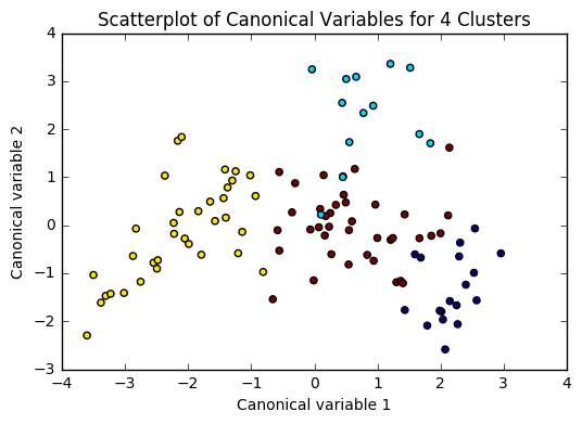
64.media.tumblr.com

Begin multiple steps to merge cluster assignment with clustering variables to examine cluster variable means by cluster.

Create a unique identifier variable from the index for the cluster training data to merge with the cluster assignment variable.

In [9]:clus_train.reset_index(level=0, inplace=True)

Create a list that has the new index variable

In [10]:cluslist = list(clus_train['index'])

Create a list of cluster assignments

In [11]:labels = list(model3.labels_)

Combine index variable list with cluster assignment list into a dictionary

In [12]:newlist = dict(zip(cluslist, labels)) print (newlist) {2: 1, 4: 2, 6: 0, 10: 0, 11: 3, 14: 2, 16: 3, 17: 0, 19: 2, 22: 2, 24: 3, 27: 3, 28: 2, 29: 2, 31: 2, 32: 0, 35: 2, 37: 3, 38: 2, 39: 3, 42: 2, 45: 2, 47: 1, 53: 3, 54: 3, 55: 1, 56: 3, 58: 2, 59: 3, 63: 0, 64: 0, 66: 3, 67: 2, 68: 3, 69: 0, 70: 2, 72: 3, 77: 3, 78: 2, 79: 2, 80: 3, 84: 3, 88: 1, 89: 1, 90: 0, 91: 0, 92: 0, 93: 3, 94: 0, 95: 1, 97: 2, 100: 0, 102: 2, 103: 2, 104: 3, 105: 1, 106: 2, 107: 2, 108: 1, 113: 3, 114: 2, 115: 2, 116: 3, 123: 3, 126: 3, 128: 3, 131: 2, 133: 3, 135: 2, 136: 0, 139: 0, 140: 3, 141: 2, 142: 3, 144: 0, 145: 1, 148: 3, 149: 2, 150: 3, 151: 3, 152: 3, 153: 3, 154: 3, 158: 3, 159: 3, 160: 2, 173: 0, 175: 3, 178: 3, 179: 0, 180: 3, 183: 2, 184: 0, 186: 1, 188: 2, 194: 3, 196: 1, 197: 2, 200: 3, 201: 1, 205: 2, 208: 2, 210: 1, 211: 2, 212: 2}

Convert newlist dictionary to a dataframe

In [13]:newclus = pd.DataFrame.from_dict(newlist, orient='index') newclus

Out[13]:0214260100113142163170192222243273282292312320352373382393422452471533543551563582593630......145114831492150315131523153315431583159316021730175317831790180318321840186118821943196119722003201120522082210121122122

105 rows × 1 columns

Rename the cluster assignment column

In [14]:newclus.columns = ['cluster']

Repeat previous steps for the cluster assignment variable

Create a unique identifier variable from the index for the cluster assignment dataframe to merge with cluster training data

In [15]:newclus.reset_index(level=0, inplace=True)

Merge the cluster assignment dataframe with the cluster training variable dataframe by the index variable

In [16]:merged_train = pd.merge(clus_train, newclus, on='index') merged_train.head(n=100)

Out[16]:indexincomeperpersonemployratefemaleemployratepolityscorealcconsumptionlifeexpectancyurbanratecluster0159-0.393486-0.0445910.3868770.0171271.843020-0.0160990.79024131196-0.146720-1.591112-1.7785290.498818-0.7447360.5059900.6052111270-0.6543650.5643511.0860520.659382-0.727105-0.481382-0.2247592329-0.6791572.3138522.3893690.3382550.554040-1.880471-1.9869992453-0.278924-0.634202-0.5159410.659382-0.1061220.4469570.62033335153-0.021869-1.020832-0.4073320.9805101.4904110.7233920.2778493635-0.6665191.1636281.004595-0.785693-0.715352-2.084304-0.7335932714-0.6341100.8543230.3733010.177691-1.303033-0.003846-1.24242828116-0.1633940.119726-0.3394510.338255-1.1659070.5304950.67993439126-0.630263-1.446126-0.3055100.6593823.1711790.033923-0.592152310123-0.163655-0.460219-0.8010420.980510-0.6448300.444628-0.560127311106-0.640452-0.2862350.1153530.659382-0.247166-2.104758-1.317152212142-0.635480-0.808186-0.7874660.0171271.155433-1.731823-0.29859331389-0.615980-2.113062-2.423400-0.625129-1.2442650.0060770.512695114160-0.6564731.9852172.199302-1.1068200.620643-1.371039-1.63383921556-0.430694-0.102586-0.2240530.659382-0.5547190.3254460.250272316180-0.559059-0.402224-0.6041870.338255-1.1776610.603401-1.777949317133-0.419521-1.668438-0.7331610.3382551.032020-0.659900-0.81098631831-0.618282-0.0155940.061048-1.2673840.211226-1.7590620.075026219171.801349-1.030498-0.4344840.6593820.7029191.1165791.8808550201450.447771-0.827517-1.731013-1.909640-1.1561120.4042250.7359771211000.974856-0.034925-0.0068330.6593822.4150301.1806761.173646022178-0.309804-1.755430-0.9368040.8199460.653945-1.6388680.2520513231732.6193200.3033760.217174-0.946256-1.0346581.2296851.99827802459-0.056177-0.2669040.2714790.8199462.0408730.5916550.63990432568-0.562821-0.3538960.0271070.338255-0.0316830.481486-0.1037773261080.111383-1.030498-1.690284-1.749076-1.3167450.5879080.999290127212-0.6582520.7286690.678765-0.464565-0.364702-1.781946-0.78874722819-0.6525281.1926250.6855540.498818-0.928876-1.306335-0.617060229188-0.662484-0.4505530.135717-1.106820-0.672255-0.147127-1.2726732..............................70140-0.594402-0.044591-0.8214060.819946-0.3157280.5125720.074137371148-0.0905570.052066-0.3190860.8199460.0936890.7235950.80625437211-0.4523170.1583900.549792-1.7490761.2768870.177913-0.140250373641.636776-0.779188-0.1697480.8199461.1084191.2715050.99128407484-0.117682-1.156153-0.5295180.9805101.8214720.5500380.5527263751750.604211-0.3248980.0882000.9805101.5903171.048938-0.287918376197-0.481087-0.0735890.393665-2.070203-0.356866-0.404628-0.287029277183-0.506714-0.808186-0.067926-2.070203-0.347071-2.051902-1.340281278210-0.628790-1.958410-1.887139-0.946256-1.297156-0.353290-1.08675317954-0.5150780.042400-0.1765360.1776910.5109430.6733710.467327380114-0.6661982.2945212.111056-0.625129-1.077755-0.229248-1.1365692814-0.5503841.5889211.445822-0.946256-0.245207-1.8114130.072358282911.575455-0.769523-0.1154430.980510-0.8426821.2795041.62732708377-0.5015740.332373-0.2783580.6593820.0545110.221758-0.28880838466-0.265535-0.0252600.305419-0.1434370.516820-0.6358011.332879385921.240375-1.243145-0.8349830.9805100.5677521.3035020.5785230862011.4545511.540592-0.733161-1.909640-1.2344700.7659211.014413187105-0.004485-1.281808-1.7513770.498818-0.8857790.3704051.418278188205-0.593947-0.1702460.305419-2.070203-0.629158-0.070373-0.8118762891540.504036-0.1605810.1696570.9805101.3846291.0649370.19511839045-0.6307520.061732-0.678856-0.625129-0.068902-1.377621-0.27991229197-0.6432031.3472771.2557550.498818-0.576267-1.199710-1.488839292632.067368-0.1992430.3597250.9805101.2298731.1133390.365916093211-0.6469130.1680550.3665130.498818-0.638953-2.020815-0.874146294158-0.422620-0.943506-0.2919340.8199461.8273490.505990-0.037060395135-0.6635950.2453810.4411820.338255-0.862272-0.018934-1.68276529679-0.6744750.6416770.1221410.338255-0.572349-2.111239-1.1223362971790.882197-0.653534-0.4344840.9805100.9810881.2578350.980609098149-0.6151691.0766361.4118810.017127-0.623282-0.626890-1.891814299113-0.464904-2.354706-1.4459120.8199460.4149550.5938830.5260393

100 rows × 9 columns

Cluster frequencies

In [17]:merged_train.cluster.value_counts()

Out[17]:3 39 2 35 0 18 1 13 Name: cluster, dtype: int64

Calculate clustering variable means by cluster

In [18]:clustergrp = merged_train.groupby('cluster').mean() print ("Clustering variable means by cluster") clustergrp Clustering variable means by cluster

Out[18]:indexincomeperpersonemployratefemaleemployratepolityscorealcconsumptionlifeexpectancyurbanratecluster093.5000001.846611-0.1960210.1010220.8110260.6785411.1956961.0784621117.461538-0.154556-1.117490-1.645378-1.069767-1.0827280.4395570.5086582100.657143-0.6282270.8551520.873487-0.583841-0.506473-1.034933-0.8963853107.512821-0.284648-0.424778-0.2000330.5317550.6146160.2302010.164805

Validate clusters in training data by examining cluster differences in internetuserate using ANOVA. First, merge internetuserate with clustering variables and cluster assignment data

In [19]:internetuserate_data = data_clean['internetuserate']

Split internetuserate data into train and test sets

In [20]:internetuserate_train, internetuserate_test = train_test_split(internetuserate_data, test_size=.3, random_state=123) internetuserate_train1=pd.DataFrame(internetuserate_train) internetuserate_train1.reset_index(level=0, inplace=True) merged_train_all=pd.merge(internetuserate_train1, merged_train, on='index') sub5 = merged_train_all[['internetuserate', 'cluster']].dropna()

In [21]:internetuserate_mod = smf.ols(formula='internetuserate ~ C(cluster)', data=sub5).fit() internetuserate_mod.summary()

Out[21]:

OLS Regression ResultsDep. Variable:internetuserateR-squared:0.679Model:OLSAdj. R-squared:0.669Method:Least SquaresF-statistic:71.17Date:Thu, 12 Jan 2017Prob (F-statistic):8.18e-25Time:20:59:17Log-Likelihood:-436.84No. Observations:105AIC:881.7Df Residuals:101BIC:892.3Df Model:3Covariance Type:nonrobustcoefstd errtP>|t|[95.0% Conf. Int.]Intercept75.20683.72720.1770.00067.813 82.601C(cluster)[T.1]-46.95175.756-8.1570.000-58.370 -35.534C(cluster)[T.2]-66.56684.587-14.5130.000-75.666 -57.468C(cluster)[T.3]-39.48604.506-8.7630.000-48.425 -30.547Omnibus:5.290Durbin-Watson:1.727Prob(Omnibus):0.071Jarque-Bera (JB):4.908Skew:0.387Prob(JB):0.0859Kurtosis:3.722Cond. No.5.90

Means for internetuserate by cluster

In [22]:m1= sub5.groupby('cluster').mean() m1

Out[22]:internetuseratecluster075.206753128.25501828.639961335.720760

Standard deviations for internetuserate by cluster

In [23]:m2= sub5.groupby('cluster').std() m2

Out[23]:internetuseratecluster014.093018121.75775228.399554319.057835

In [24]:mc1 = multi.MultiComparison(sub5['internetuserate'], sub5['cluster']) res1 = mc1.tukeyhsd() res1.summary()

Out[24]:

Multiple Comparison of Means - Tukey HSD,FWER=0.05group1group2meandifflowerupperreject01-46.9517-61.9887-31.9148True02-66.5668-78.5495-54.5841True03-39.486-51.2581-27.7139True12-19.6151-33.0335-6.1966True137.4657-5.76520.6965False2327.080817.461736.6999True

The elbow curve was inconclusive, suggesting that the 2, 4, 6, and 8-cluster solutions might be interpreted. The results above are for an interpretation of the 4-cluster solution.

In order to externally validate the clusters, an Analysis of Variance (ANOVA) was conducting to test for significant differences between the clusters on internet use rate. A tukey test was used for post hoc comparisons between the clusters. Results indicated significant differences between the clusters on internet use rate (F=71.17, p<.0001). The tukey post hoc comparisons showed significant differences between clusters on internet use rate, with the exception that clusters 0 and 2 were not significantly different from each other. Countries in cluster 1 had the highest internet use rate (mean=75.2, sd=14.1), and cluster 3 had the lowest internet use rate (mean=8.64, sd=8.40).

[arijit123]

Data Management and Visualization Assignment 1

My name is Arijit Banerjee and this blog is a part of Data Management and Visualization course on coursera. The submission of the assignments will be in the form of blogs. So I choose medium as my medium of assignment.

Assignment 1

In assignment 1, we've to choose dataset on which we've to work for the whole course. The five law books are given through which we've to elect a subcategory and two motifs/ variable on which we want to work.

STEP 1 Choose a data set that you would like to work with.

After reviewing five codebooks, I've decide to go with “ portion of the GapMinder ”. This data includes one time of multitudinous country- position pointers of health, wealth and development. I want work on health issue is the main reason to choose this text. In moment’s world, the average life expectation is increased. But some intoxication cause early death.

STEP 2. Identify a specific content of interest

As I want to explore the average life expectation including some intoxication, I would like to go with alcohol consumption and life expectation. As the alcohol consumption is so pernicious to health I would like to aim this issue to how important it’s dangerous. So I ’m considering how the alcohol consumption will prompt to health and other parameters or which parameters are related to to alcohol consumption.

STEP 3. Prepare a codebook of your own

As, GapMinder includes variables piecemeal from health( wealth, development). So then I ’m considering only incomeperperson, alcconsumption and lifeexpectancy as variables.

Image

STEP 4. Identify a alternate content that you would like to explore in terms of its association with your original content.

The alternate content which I would like to explore is urbanrate. While looking at the codebook, I allowed that there might be possibility that civic rate is connected to alcohol consumption. We can see in civic area, people are less apprehensive of their health and consume further toxic.

STEP 5. Add questions particulars variables establishing this alternate content to your particular codebook.

Is there any relation between civic rate and alcohol consumption?

Is there any relation between life expectation and alcohol consumption?

Is there any relation between Income and alcohol consumption?

The final Codebook

Image

STEP 6. Perform a literature review to see what exploration has been preliminarily done on this content

For the relation between urbanrate and alcohol consumption, I search so much on google scholar but there isn't a single paper on it. When I had hunt on google itself, I got to know that there's nor direct relation between this two. The relation as in terms of stress and culture. Those can be in megacity and civic are also. So I do n’t have to consider this term( urbanrate). For the relation between life expectation and alcohol consumption, I got lots of papers on it so do with income and alcohol consumption. Then are many papers and overview of their content.

1. Continuance income patterns and alcohol consumption probing the association between long- and short- term income circles and drinking( 1)

Overview In this paper, authors estimated the relationship between long- term and short- term measures of income. They used the data of US Panel Study on Income Dynamics. They also gave conclusion like the low income associated with heavy consumption. “ Continuance income patterns may have an circular association with alcohol use, intermediated through current socioeconomic position. ”( 1)

A Review of Expectancy Theory and Alcohol Consumption( 2)

According to their study, “ expectation manipulations and alcohol consumption three studies in the laboratory have shown that adding positive contemplations through word priming increases posterior consumption and two studies have shown that adding negative contemplations decreases it ”( 2)

2. Alcohol- related mortality by age and coitus and its impact on life expectation Estimates grounded on the Finnish death register( 3)

In this composition, the author studied presumptive results on the connection between alcohol- related mortality and age and coitus. Then are many statistics, “ According to the results, 6 of all deaths were alcohol related. These deaths were responsible for a 2 time loss in life expectation at age 15 times among men and0.4 times among women, which explains at least one- fifth of the difference in life contemplations between the relations. In the age group of 15 – 49 times, over 40 of all deaths among men and 15 among women were alcohol related. In this age group, over 50 of the mortality difference between the relations results from alcohol- related deaths ”( 3)

STEP 7. Grounded on your literature review, develop a thesis about what you believe the association might be between these motifs. Be sure to integrate the specific variables you named into the thesis.

After exploring similar papers, they're enough to establish the correlation between alcohol consumption and life expectation and also with Income( piecemeal from these three). After certain observation, following are my thesis

• The alcohol consumption is largely identified with life expectation.

• The social culture, group of people associated with person, stress and Income have direct correlation with alcohol consumption.

• Civic rate isn't directly connected to alcohol consumption.

Final Codebook

Reference

Cerdá, Magdalena, etal. “ Continuance Income Patterns and Alcohol Consumption probing the Association between Long- and Short- Term Income Circles and Drinking. ” Social Science & Medicine,vol. 73,no. 8, 2011,pp. 1178 – 1185., doi10.1016/j.socscimed.2011.07.025.

2) Jones, BarryT., etal. “ A Review of Expectancy Theory and Alcohol Consumption. ” Dependence,vol. 96,no. 1, 2001,pp. 57 – 72., doi10.1046/j. 1360 –0443.2001.961575.x.

3) Makela,P. “ Alcohol- Related Mortality by Age and Sex and Its Impact on Life Expectancy. ” The European Journal of Public Health,vol. 8,no. 1, 1998,pp. 43 – 51., doi10.1093/ eurpub/8.1.43.

#arijit#Data Management and Visualization#coursera

[sreyakotagiri]

Choosing a dataset, developing a research question and then creating a personal codebook

Dataset chosen:Gapminder

Research Question:Is co2 emissions associated with the urban rate?

I would like to study how the co2 emissions affect the urban rate. The variables documenting to this topic are co2 emissions and the urbanrate.

[varshadarimadugu]

Choosing a Data set, developing a research question and creating a personal codebook

Data Set chosen: Gapminder

Research Question: Is the Co2 emission rate associated with urban rate.

I would like to study how the Co2 emission rate affected by the urban population rate. The attributes I would like to consider are urbanrate and co2emissions.

[anotherdataanalyst]

Analysis of some Gapminder data (part3)

I revised the first code and added the first visual features.

You can find code and output below, including a short summary.

Data management decisions have been docuemtned in the code comments:

deletion of incomplete data

different clustering in order to have meaningful data

CODE:

#import necessary libraries

import pandas as pd import numpy as np

#import data set and check number of observations and variables

data = pd.read_csv('gapminder.csv', low_memory=False) number_of_orig_row = len(data) print('Some data set information:') print(len(data.columns), 'observed variables') print(number_of_orig_row, 'observations')

#convert necessary variables to numeric values

#and remove incomplete missing data

data['urbanrate']=pd.to_numeric(data['urbanrate'],'coerce') data['co2emissions']=pd.to_numeric(data['co2emissions'],'coerce') data['lifeexpectancy']=pd.to_numeric(data['lifeexpectancy'],'coerce') data.dropna(subset=['urbanrate','co2emissions','lifeexpectancy'], inplace=True)

#calculate some useful data

co2_max = data['co2emissions'].max() missing_data = number_of_orig_row - len(data) print(missing_data,'observations will be deleted since not all variables were filled with values') print()

#used variables do not include recurrent values,

#creating frequency tables out of this raw data will not help much

#instead variable data will be clustered in groups

#that can be used for frequency anaylsis

#'urbanrate' can be clustered by <25% / <50% / <75% / <100%

#'co2emissions' can be clustered by < co2_max/10000, < co2_max/1000, < co2_max/100, > co2_max/100

#'lifeexpectation' can be clustered by <60, <70, <80, <90

data['urbanrate_cl'] = data['urbanrate'].apply(lambda x: 'ur25' if x < 25 else ('ur50' if x < 50 else ('ur75' if x < 75 else 'ur100'))) data['co2emissions_cl'] = data['co2emissions'].apply(lambda x: 'ce10000' if x < co2_max/10000 else ('ce1000' if x < co2_max/1000 else ('ce100' if x < co2_max / 100 else 'ce_max'))) data['lifeexpectancy_cl'] = data['lifeexpectancy'].apply(lambda x: 'le60' if x < 60 else ('le70' if x < 70 else ('le80' if x < 80 else 'le90')))

#create and print frequency tables (with labels)

c_ur = data['urbanrate_cl'].value_counts(sort=False, normalize=False) p_ur = 100 * data['urbanrate_cl'].value_counts(sort=False, dropna=False, normalize=True) print('The count of the clustered values of variable "urbanrate" is:') print(c_ur) print() print('while the relative frequency (percentage) is in %:') print(p_ur) c_ce = data['co2emissions_cl'].value_counts(sort=False, normalize=False) p_ce = 100 * data['co2emissions_cl'].value_counts(sort=False, dropna=False, normalize=True) print() print('The count of the clustered values of variable "co2emissions" is:') print(c_ce) print() print('while the relative frequency (percentage) is in %:') print(p_ce) print() c_le = data['lifeexpectancy_cl'].value_counts(sort=False, normalize=False) p_le = 100 * data['lifeexpectancy_cl'].value_counts(sort=False, dropna=False, normalize=True) print('The count of the clustered values of variable "lifeexpectancy" is:') print(c_le) print() print('while the relative frequency (percentage) is in %:') print(p_le)

c_ur.plot(kind='bar') c_ce.plot(kind='bar') c_le.plot(kind='bar')

OUTPUT:

Some data set information: 16 observed variables 213 observations 32 observations will be deleted since not all variables were filled with values

The count of the clustered values of variable "urbanrate" is: ur25 19 ur50 54 ur75 69 ur100 39 Name: urbanrate_cl, dtype: int64

while the relative frequency (percentage) is in %: ur25 10.497238 ur50 29.834254 ur75 38.121547 ur100 21.546961 Name: urbanrate_cl, dtype: float64

The count of the clustered values of variable "co2emissions" is: ce1000 66 ce100 47 ce_max 33 ce10000 35 Name: co2emissions_cl, dtype: int64

while the relative frequency (percentage) is in %: ce1000 36.464088 ce100 25.966851 ce_max 18.232044 ce10000 19.337017 Name: co2emissions_cl, dtype: float64

The count of the clustered values of variable "lifeexpectancy" is: le60 37 le80 85 le90 22 le70 37 Name: lifeexpectancy_cl, dtype: int64

while the relative frequency (percentage) is in %: le60 20.441989 le80 46.961326 le90 12.154696 le70 20.441989 Name: lifeexpectancy_cl, dtype: float64

SHORT SUMMARY

Calculated relative frequencies indicates following:

life expectation gets its highest value in the band 70 till 80 years, showing surprisingly a minimum in the band 60 till 70.

urban rate has its highest frequency between 50 and 70%, nevertheless the contiguous bands have also high values. Less then 25% has the lowest values.

co2 emissions are very different, therefore the clusters have been chosen using scale factors (100/1000/10000 times). Countries with the lowest values have negligible emissions in comparison with the others.

[dataanalyst75]

Testing a multiple regression model for the likely association between urban population referring to people living in urban areas and internet users which access to the worldwide network (adjusting for potential confounding factors)

Multiple regression SAS output from "Evaluating model fit for evidence of any misspecification"

- see https://www.tumblr.com/dataanalyst75/759717025183629313/testing-a-multiple-regression-model-for-the-likely?source=share for description

SAS code

/*Program for GAPMINDER data set*/ PROC IMPORT DATAFILE ='/home/u63783903/my_courses/gapminder_pds.csv' OUT = imported REPLACE; RUN; DATA new; set imported; /* the gapminder csv dataset is being uploaded and imported to the SAS - the dataset is being read and prepared for use */

/* List of quantitative explanatory variables containing the primary explanatory variable - intenet users' rate and other likely confounding factors */ LABEL urbanrate = "Gross Domestic Product per capita in constant 2000 US$" Internetuserate ="Internet users (per 100 people)" employrate = "Percentage of total populationthat has been employed during a given year" polityscore = "2009 Democracy score (Polity) - Overall polity score from the Polity IV dataset";

************************************************************************************************************** DATA MANAGEMENT **************************************************************************************************************;

if urbanrate ne . and Internetuserate ne . and employrate ne . and polityscore ne . ; /* Only observations of likely predictors with values not equal to blank are being considered for present analysis */

**************************************************************************************************** END DATA MANAGEMENT ****************************************************************************************************;

PROC MEANS; var Internetuserate urbanrate employrate polityscore; run; * the mean values serve to center afterwards the primary explanatory variable and likely confounding factors by subtracting the mean value from the actual value for each observation;

************************************************************************************************************** ADDITIONAL DATA MANAGEMENT to create a new temporary data set to handle the centered explanatory variables **************************************************************************************************************; data new2; set new; * additional data management needed to create a new temporary data set;

**************************************************************************************************** END DATA MANAGEMENT ****************************************************************************************************;

* centered variables being used in the regression analysis; Internetuserate_c = Internetuserate-32.5051688; employrate_c = employrate-59.2802632; urbanrate_c = urbanrate - 56.8410778; polityscore_c=polityscore-3.7960526;

run;

* check coding to assess whether the variables are properly centered by calculating the mean of each centered variable using the means procedure; PROC MEANS; var Internetuserate_c employrate_c polityscore_c; run;

**************************************************************************************************** POLYNOMIAL REGRESSION ****************************************************************************************************; * it has been considered a curvilinear relationship between internet users’ and urban rate in the multi regression analysis, rather than a linear. That means: i.e. a curve best captures the non-linear nature of the association among the variables in question: in other words, the expected or predicted values provided by adding a second order polynomial term of internet users’ rate are closer to the actual observed values of urban rate; PROC glm; model urbanrate = Internetuserate_c Internetuserate_c*Internetuserate_c /solution clparm; run;

* scatterplot for x variable, Internetuserate and y urbanrate with linear and quadratic regression line showing that a curvilinear / quadratic polynomial relationship between internet users’ and urban rate best captures the non-linear nature of the association among the variables in question: the 95% confidence interval for the regression line being printed as well; proc sgplot; reg x=Internetuserate y=urbanrate / lineattrs=(color=blue thickness=2) degree=1 clm; reg x=Internetuserate y=urbanrate / lineattrs=(color=green thickness=2) degree=2 clm; yaxis label="Urban population referring to people living in urban areas"; xaxis label="Internet users (per 100 people)"; run;

* As the coefficients for the linear and quadratic internet users’ rate remain significant after adjusting for employment rate, and employment rate is also statistically significant (p-value = 0.0198), they all have been taken into account for the regression model equation; PROC glm; model urbanrate = Internetuserate_c Internetuserate_c*Internetuserate_c employrate_c /solution clparm; run;

************************************************************************************************* EVALUATING MODEL FIT *************************************************************************************************; /* Model residuals via residual plots to examine any violation of the assumptions of the linear regression analysis (visual evaluation of specification errors)

diagnostic plots being printed out in addition to the statistics for the regression model: plots being unpacked into separate graphs.

Q-Q Plot to evaluate the assumption that the residuals from the regression model are normally distributed; Residual plots for each observation at different values of individual explanatory variables; Leverage plot to identify observations that have unusually large influence on the estimation of the predicted value of urban rate

The primary explanatory variable - internet users' rate and employ rate (predictor) have been taking into account for the regression model, as these explanatory variables are statistical significantly associated with urban rate */ PROC glm PLOTS(unpack)=all; model urbanrate = Internetuserate_c Internetuserate_c*Internetuserate_c employrate_c /solution clparm; output residual=res student=stdres out=results; run;

* plot of standardized residuals for each observation to evaluate the overall fit of the predicted values of the response variable to the observed values, and look for outliers. A plot of the standardized residuals for each of the observations is being examined ; proc gplot; label stdres="Standardized Residual" country="Country"; plot stdres*country/vref=0; run;

* using proc reg to get a partial regression plot; *Partial regression residual plots are used to assess the contribution of each individual explanatory variable to the model fit, controlling for the other explanatory variables; * calculate quadratic terms; data partial; set new2; Internetuserate2=Internetuserate_c*Internetuserate_c ; run;

*partial regression plot; PROC reg plots=partial; model urbanrate=Internetuserate Internetuserate2 employrate/partial; run;

[datasicienceprojectweek2]

Assignment Week 2: Running Your First Program

TITLE

Impact of Employment on Mental Health Globally from Gapminder Data: Analyzing the Relationship between employment rates and suicide rates across countries?

Refined Research Question:

How do employment rates impact suicide rates globally, and does this association change when considering income per person, urbanization, and alcohol consumption?

NOTE: The Data presented and analyzed based on the Data presented by Gapminder Dataset provided in the course material.

Explotary Data Analysis. *We will explore the Gapminder datasets and try to gain insihts about the data using basic statistics metrics using python

Conclusion:

We saw there are 213 observations and 16 columns(features) provided in the gapminder dataset as per the course material There is one categorical column "country" and the rest are numeric variables based on my reserach question: Impact of Employment on Mental Health Globally from Gapminder Data: Analyzing the Relationship between employment rates and suicide rates across countries? Refined Research Question: How do employment rates impact suicide rates globally, and does this association change when considering income per person, urbanization, and alcohol consumption?

below are the list of variables that I will be considering for my research project: employrate suicideper100th incomeperperson urbanrate alcconsumption female employrate (additional)

Data Processing/Cleaning:

On doing basic analysis and EDA we found that there were around 50 records which had one or the other missing data which consitituted to around 23% missing data. To handle missing data, we first added a region column to map the countries to respective regions Then using the region we used the group mean to replace the the missing data.

Frequency/Distribution:

Looking at the frequency distribution of the three variables of interest: 1. incomeperperson: It is seen that majority of the countries mean incomeperperon is is up to 10000 USD with few falling between 10K to 40K and wee also see their are outliers above 40K. Data is right skewed. 2. Suiciderate is showing with majority of the countries falling with a mean of 9.57 and std of 6.07 and we see there are some outliers 3. employrate shows that in majority of the countries around 58.72 % of population age above 15+ are employed with std of 9.8. 4.

We will have to do more data processing to see how best we can use the data to gain further insights and relationships between the variables.

[dspoject101]

Assignment Week 1: Impact of Employment on Mental Health Globally.

Data Set: GAPMINDER

Motivation: The relationship between employment rates and mental health, specifically suicide rates, is a critical area of research that addresses fundamental issues of economic stability, social welfare, and public health. Understanding how employment status impacts mental well-being is essential for developing effective policies and interventions that can mitigate the adverse effects of unemployment and economic downturns on individuals and communities.

Research Question:

Is there an association between employment rates and suicide rates across countries?

Refined Research Question:

How do employment rates impact suicide rates globally, and does this association change when considering income per person, urbanization, and alcohol consumption?

Key words used: Unemployment + mental health + suicide + alcohol + urbanisation

Literature Review References:

Nordt, C., Warnke, I., Seifritz, E., & Kawohl, W. (2015). "Modelling suicide and unemployment: a longitudinal analysis covering 63 countries, 2000–2011." The Lancet Psychiatry, 2(3), 239-245.

This study explores the relationship between unemployment rates and suicide rates, providing evidence of a significant correlation, and emphasizes the importance of economic factors in mental health outcomes.

Stuckler, D., Basu, S., Suhrcke, M., Coutts, A., & McKee, M. (2009). "The public health effect of economic crises and alternative policy responses in Europe: an empirical analysis." The Lancet, 374(9686), 315-323.

This research examines the impact of economic crises on public health, including mental health outcomes like suicide rates, highlighting the influence of employment status on these outcomes.

Blakely, T. A., Collings, S. C. D., & Atkinson, J. (2003). "Unemployment and suicide. Evidence for a causal association?" Journal of Epidemiology & Community Health, 57(8), 594-600.

This paper discusses the potential causal relationship between unemployment and suicide, contributing to the understanding of how economic and employment factors affect mental health.

Chang, S. S., Gunnell, D., Sterne, J. A., Lu, T. H., & Cheng, A. T. (2009). "Was the economic crisis 1997-1998 responsible for rising suicide rates in East/Southeast Asia? A time-trend analysis for Japan, Hong Kong, South Korea, Taiwan, Singapore and Thailand." Social Science & Medicine, 68(7), 1322-1331.

This study analyzes the rise in suicide rates during economic crises in East/Southeast Asia, underscoring the relationship between employment and mental health in different cultural contexts.

Kawachi, I., & Wamala, S. (Eds.). (2006). "Globalization and Health." Oxford University Press.

This book covers various aspects of globalization and their impact on health, including how changes in employment patterns influence mental health and suicide rates worldwide.

Hypothesis:

Null Hypothesis (H0): There is no significant association between employment rates and suicide rates across countries.

Alternative Hypothesis (H1): Higher employment rates are associated with lower suicide rates across countries, even when controlling for income per person, urbanization, and alcohol consumption.

Codebook and Variables:

Group 1: Employment Rates

employrate: This variable measures the employment rate in each country, representing the percentage of the working-age population that is employed.

Group 2: Suicide Rates

suicideper100th: This variable measures the rate of suicides per 100,000 people in each country.

Control Variables:

incomeperperson: This variable measures the average income per person, representing economic status.

urbanrate: This variable measures the percentage of the population living in urban areas, representing urbanization levels.

alcconsumption: This variable measures the average alcohol consumption per person, representing potential influences on mental health.

References:

Nordt, C., Warnke, I., Seifritz, E., & Kawohl, W. (2015). Modelling suicide and unemployment: a longitudinal analysis covering 63 countries, 2000–2011. The Lancet Psychiatry, 2(3), 239-245.

Stuckler, D., Basu, S., Suhrcke, M., Coutts, A., & McKee, M. (2009). The public health effect of economic crises and alternative policy responses in Europe: an empirical analysis. The Lancet, 374(9686), 315-323.

Blakely, T. A., Collings, S. C. D., & Atkinson, J. (2003). Unemployment and suicide. Evidence for a causal association? Journal of Epidemiology & Community Health, 57(8), 594-600.

Chang, S. S., Gunnell, D., Sterne, J. A., Lu, T. H., & Cheng, A. T. (2009). Was the economic crisis 1997-1998 responsible for rising suicide rates in East/Southeast Asia? A time-trend analysis for Japan, Hong Kong, South Korea, Taiwan, Singapore and Thailand. Social Science & Medicine, 68(7), 1322-1331.

Kawachi, I., & Wamala, S. (Eds.). (2006). Globalization and Health. Oxford University Press.

[nycegreedy]

NYCE GREEDY - Put The Money First ft Mackin Fat (Official Visualizer) #detroit

NYCE GREEDY - Put The Money First ft Mackin Fat (Official Visualizer) #detroit https://www.youtube.com/watch?v=9TyCTQHY2gk AIR GREEDY Explore Nyce Greedy’s powerful anthem ‘Put the Money First’ detailing the pitfalls of hustling for love and the perils of placing women above financial priorities. Discover how focusing on wealth transforms lives, contrasting the hardships of misplaced priorities with the rewards of financial dedication. Stream now for a compelling narrative on urban realities and success.” #AIRGREEDY #PutTheMoneyFirst #NyceGreedy #UrbanRealities #FinancialSuccess #HustleForSuccess #LoveVsWealth #HipHopNarratives #RapAnthem #MoneyMoves #SuccessStories ⭐⭐⭐If you love the hottest hip-hop and rap music tracks, you don't want to miss out on the latest updates. By hitting that subscribe button, you'll stay up-to-date with the newest releases: https://www.youtube.com/@NyceGreedy/?sub_confirmation=1 ⭐ ⭐ ⭐ Audio Music is currently on your favorite platforms: 👉AppleMusic:https://ift.tt/gT6tYCZ 🔗 Stay Connected With Me. 👉Instagram: https://ift.tt/nz5uf6d 👉Threads: https://ift.tt/OR9Bkuz 👉Twitter (X): https://twitter.com/NyceGreedy ✅ For Business Inquiries: nycegreedy@gmail.com ============================= ✅ Other Videos You Might Be Interested In Watching: 📀 3RD BLOCK WAY Freestyle https://www.youtube.com/watch?v=nX0pk2XsOhc 📀 Nyce Greedy ft. Payroll Giovanni - 3rd To Da Moor (Official Music Video) https://www.youtube.com/watch?v=UJSfs1axqzg 📀 Nyce Greedy - Arm Challenge (Official Music Video) https://www.youtube.com/watch?v=DdUda53LgCE ============================= ✅ About Nyce Greedy. Detroit-born and raised, Nyce Greedy is a versatile rapper who stays true to his Fenkell Avenue roots through his unique perspective and raw lyricism. With a relentless drive and passion for his craft, Nyce Greedy continues to push boundaries and inspire listeners with his artistry. For Collaboration and Business inquiries, please use the contact information below: 📩 Email: nycegreedy@gmail.com 🔔Are you a fan of gangster rap and original Detroit hip-hop? If so, don't miss out on the latest music tracks! Hit that subscribe button and stay up-to-date with the raw lyricism & latest releases:https://www.youtube.com/@NyceGreedy/?sub_confirmation=1 ================================= ⚠️Disclaimer: I do not accept any liability for any loss or damage incurred from you acting or not acting as a result of watching any of my publications. You acknowledge that you use the information I provide at your own risk. Do your research. Copyright Notice: This video and my YouTube channel contain dialogue, music, and images that are the property of Nyce Greedy. You are authorized to share the video link and channel and embed this video in your website or others as long as a link back to my YouTube channel is provided. © Nyce Greedy via Nyce Greedy https://www.youtube.com/channel/UCrBiN-9q0_my5Z60MyMsb-Q July 11, 2024 at 11:34AM

[jorge-quintero]

Getting Your Research Project Started

GapMinder

Análisis de Desarrollo Económico: Comparar el PIB y las tasas de empleo entre diferentes países para evaluar el progreso económico.

incomeperperson (2010 GDP per capita in constant 2000 US$) femaleemployrate (2007 female employees age 15+ (% of population)) employrate (2007 total employees age 15+ (% of population)) lifeexpectancy (2011 life expectancy at birth (years)) Internetuserate (2010 Internet users (per 100 people)) urbanrate (2008 urban population (% of total))

4.salud y el bienestar de la población.

5.incomeperperson (2010 GDP per capita in constant 2000 US$) femaleemployrate (2007 female employees age 15+ (% of population))

6.Canales, A. B. A. (2021). Enfermería: Comprometida con la salud y el bienestar de la población. Universidad Juárez del Estado de Durango.

7.El desarrollo económico de un país está positivamente asociado con la salud y el bienestar de su población. Específicamente, se espera que los países con mayor Producto Interno Bruto (PIB) per cápita y tasas de empleo más altas tengan mayores expectativas de vida, menor prevalencia de VIH y cáncer, menores tasas de suicidio, y mayores niveles de consumo de electricidad residencial y uso de Internet

[sidslash918]

Data Analysis Tools - Week 4 Assignment

We are using the Gapminder dataset in our assignment. We will find out the association between the variables listed below:

incomeperperson 2010 Gross Domestic Product per capita in constant 2000 US$. The inflation but not the differences in the cost of living. 

alcconsumption 2008 alcohol consumption per adult (age 15+), litres Recorded and estimated average alcohol consumption, adult (15+) per capita consumption in litres pure alcohol.

oilperperson 2010 oil Consumption per capita (tonnes per year and person).

hivrate 2009 estimated HIV Prevalence % - (Ages 15-49) Estimated number of people living with HIV per 10.

employrate 2007 total employees age 15+ (% of population) Percentage of total population, age above 15, that has been employed during the given year.

polityscore 2009 Democracy score (Polity) Overall polity score from the Polity IV dataset, calculated by subtracting an autocracy score from a democracy score. The summary measure of a country's democratic and free nature. -10 is the lowest value, 10 the highest.

Syntax of the code used:

Libname data '/home/u47394085/Data Analysis and Interpretation';

Proc Import Datafile='/home/u47394085/Data Analysis and Interpretation/gapminder.csv' Out=data.Gapminder Dbms=csv replace; Run;

Data Gapminder; Set data.Gapminder; Format IncomeGroup $30. PoliticalStability $20. Urbanization $10. Alcoholism $10.; If incomeperperson=. Then IncomeGroup='NA'; Else If incomeperperson>0 and incomeperperson<=1500 Then IncomeGroup='Lower'; Else If incomeperperson>1500 and incomeperperson<=4500 Then IncomeGroup='Lower Middle'; Else If incomeperperson>4500 and incomeperperson<=15000 Then IncomeGroup='Upper Middle'; Else IncomeGroup='Upper';

If polityscore=. Then PoliticalStability='NA'; Else If polityscore<5 Then PoliticalStability='Unstable'; Else PoliticalStability='Stable';

If urbanrate=. Then Urbanization='NA'; Else If urbanrate<50 Then Urbanization='Low'; Else Urbanization='High';

If alcconsumption=. Then Alcoholism='NA'; Else If alcconsumption<3 Then Alcoholism='Low'; Else If alcconsumption<=6 Then Alcoholism='Medium'; Else Alcoholism='High';

Run;

/* Testing a Potential Moderator / / ANOVA Studying the association between PoliticalStability (Explanatory Variable) and Hivrate (Dependent Variable) factoring in the confounding variable Incomegroup */

Proc Sort Data=Gapminder; By IncomeGroup; Run;

Proc Anova; Class PoliticalStability; Model hivrate=PoliticalStability; Means PoliticalStability; By IncomeGroup; Where PoliticalStability ne 'NA' AND hivrate ne . AND incomeperperson ne .; Run;

Results:

Since, the p value<0.05, it signifies that there is an association between Political Stability and Hivrate only for countries in "Upper Middle" income group with mean value for hivrate being 2.55 for politically unstable and 0.40 for stable countries. In an nutshell, hivrate is more for politically unstable countries with incomeperson in the range $4500 and $15000.

/* CHI SQUARE Studying the association between Incomegroup (Explanatory Variable) and Alcoholism (Dependent Variable) factoring in the confounding variable PoliticalStability */

Proc Freq Data=Gapminder; Tables Alcoholism*Incomegroup / CHISQ; By PoliticalStability; Where PoliticalStability ne 'NA' AND Alcoholism ne 'NA' AND incomeperperson ne .; Run;

/Post Hoc Test with Bonferroni Adjustment (p value is 0.05/6 = 0.00833333333)/ Proc Freq Data=Gapminder; Tables Alcoholism*Incomegroup / CHISQ; Where Incomegroup IN ('Lower', 'Lower Middle'); Run;

Proc Freq Data=Gapminder; Tables Alcoholism*Incomegroup / CHISQ; Where Incomegroup IN ('Lower', 'Upper Middle'); Run;

Proc Freq Data=Gapminder; Tables Alcoholism*Incomegroup / CHISQ; Where Incomegroup IN ('Lower', 'Upper'); Run;

Proc Freq Data=Gapminder; Tables Alcoholism*Incomegroup / CHISQ; Where Incomegroup IN ('Lower Middle', 'Upper Middle'); Run;

Proc Freq Data=Gapminder; Tables Alcoholism*Incomegroup / CHISQ; Where Incomegroup IN ('Lower Middle', 'Upper'); Run;

Proc Freq Data=Gapminder; Tables Alcoholism*Incomegroup / CHISQ; Where Incomegroup IN ('Upper Middle', 'Upper'); Run;

Results:

Interpretation: Since the p>0.00833, there is no association between alcoholism and incomegroups Lower Middle and Upper Middle countries. for politically stable countries. As per the data, as the income rises so does the alcoholism.

/* Pearson Correlation Studying the association between employrate (Explanatory Variable) and oilperperson (Dependent Variable) factoring in the confounding variable IncomeGroup

*/

Proc Sort Data=Gapminder; By IncomeGroup; Run;

Proc Corr Data=Gapminder; Var employrate oilperperson; By IncomeGroup; Where IncomeGroup ne 'NA' AND employrate ne . AND oilperperson ne .; Run;

Results:

Interpretation:

Since the p <0.05 for all of the income groups, we can conclude that there is no association between employrate and oilperperson.