sandeepsrinivas19 - Tumblr blog

sandeepsrinivas19 · 6 years

Text

House Price Classification (1-6) using Lasso Regression

House Price Classification

The objective is to classify the price of a house with the given parameters into the following price classes: 1 = <$250,000 2 = $250,000-$500,000 3 = $500,000-$750,000 4 = $750,000-$1,000,000 5 = $1,000,000-$1,250,000 6 = >$1,250,000

and identify the various parameters responsible for the pricing. The data is for various parameters (predictors) like number of bedrooms, sqft living area, number of bathrooms, whether the house has a view or not etc (from online source) is fed into the classification regression model. Target variable is the price_class of the house.

Each variable was standardised to have a mean of 0 and a standard deviation of 1 while pre-processing. A k=10 fold cross-validation technique was used to test the model.

Code #########################

#from pandas import Series, DataFrame import os import pandas as pd import numpy as np import matplotlib.pylab as plt from sklearn.cross_validation import train_test_split from sklearn.linear_model import LassoLarsCV

os.chdir("A:\ML Coursera") #Load the dataset data = pd.read_csv("home_data4.csv")

#upper-case all DataFrame column names data.columns = map(str.upper, data.columns)

# Data Management data_clean = data.dropna()

#select predictor variables and target variable as separate data sets predvar= data_clean[['BEDROOMS', 'BATHROOMS', 'SQFT_LIVING', 'SQFT_LOT', 'FLOORS', 'WATERFRONT', 'VIEW', 'CONDITION', 'GRADE', 'SQFT_ABOVE', 'SQFT_BASEMENT', 'YR_BUILT' ]]

target = data_clean.PRICE_CLASS

# standardize predictors to have mean=0 and sd=1 predictors=predvar.copy() from sklearn import preprocessing predictors['BEDROOMS']=preprocessing.scale(predictors['BEDROOMS'].astype('float64')) predictors['BATHROOMS']=preprocessing.scale(predictors['BATHROOMS'].astype('float64')) predictors['SQFT_LIVING']=preprocessing.scale(predictors['SQFT_LIVING'].astype('float64')) predictors['SQFT_LOT']=preprocessing.scale(predictors['SQFT_LOT'].astype('float64')) predictors['FLOORS']=preprocessing.scale(predictors['FLOORS'].astype('float64')) predictors['WATERFRONT']=preprocessing.scale(predictors['WATERFRONT'].astype('float64')) predictors['VIEW']=preprocessing.scale(predictors['VIEW'].astype('float64')) predictors['CONDITION']=preprocessing.scale(predictors['CONDITION'].astype('float64')) predictors['GRADE']=preprocessing.scale(predictors['GRADE'].astype('float64')) predictors['SQFT_ABOVE']=preprocessing.scale(predictors['SQFT_ABOVE'].astype('float64')) predictors['SQFT_BASEMENT']=preprocessing.scale(predictors['SQFT_BASEMENT'].astype('float64')) predictors['YR_BUILT']=preprocessing.scale(predictors['YR_BUILT'].astype('float64'))

predictors.head() # split data into train and test sets pred_train, pred_test, tar_train, tar_test = train_test_split(predictors, target, test_size=.3, random_state=123)

# specify the lasso regression model model=LassoLarsCV(cv=10, precompute=False).fit(pred_train,tar_train)

# print variable names and regression coefficients dict(zip(predictors.columns, model.coef_))

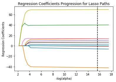
# plot coefficient progression m_log_alphas = -np.log10(model.alphas_) ax = plt.gca() plt.plot(m_log_alphas, model.coef_path_.T) plt.axvline(-np.log10(model.alpha_), linestyle='--', color='k', label='alpha CV') plt.ylabel('Regression Coefficients') plt.xlabel('-log(alpha)') plt.title('Regression Coefficients Progression for Lasso Paths')

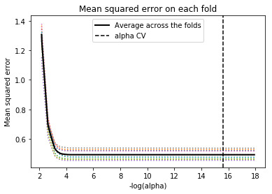
# plot mean square error for each fold m_log_alphascv = -np.log10(model.cv_alphas_) plt.figure() plt.plot(m_log_alphascv, model.cv_mse_path_, ':') plt.plot(m_log_alphascv, model.cv_mse_path_.mean(axis=-1), 'k', label='Average across the folds', linewidth=2) plt.axvline(-np.log10(model.alpha_), linestyle='--', color='k', label='alpha CV') plt.legend() plt.xlabel('-log(alpha)') plt.ylabel('Mean squared error') plt.title('Mean squared error on each fold')

# MSE from training and test data from sklearn.metrics import mean_squared_error train_error = mean_squared_error(tar_train, model.predict(pred_train)) test_error = mean_squared_error(tar_test, model.predict(pred_test)) print ('training data MSE') print(train_error) print ('test data MSE') print(test_error)

# R-square from training and test data rsquared_train=model.score(pred_train,tar_train) rsquared_test=model.score(pred_test,tar_test) print ('training data R-square') print(rsquared_train) print ('test data R-square') print(rsquared_test)

#########################

Output:

{'BEDROOMS': -0.051115370744155196, 'BATHROOMS': 0.11210926212354395, 'SQFT_LIVING': 0.32651387620252414, 'SQFT_LOT': -0.00865938319608584, 'FLOORS': 0.08635931610792122, 'WATERFRONT': 0.059669258580336657, 'VIEW': 0.11322348584018982, 'CONDITION': 0.0541793720936317, 'GRADE': 0.5706466464368843, 'SQFT_ABOVE': 0.0, 'SQFT_BASEMENT': 0.02533279918612259, 'YR_BUILT': -0.3439055814902168}

training data MSE 0.4905109604220459 test data MSE 0.48521148751529647

training data R-square 0.6247653438966141 test data R-square 0.6385205011430025

Interpretation: As we can see from the model output, some of the parameters' coefficients has been shrunk to very low values (like Sqft_above and Sqft_lot) indicating that these are not particularly influential in the pricing of the house.

Sqft_living, Grade (describing the quality of the material) and the year built have the highest coefficients indicating that these are the most influential parameters. This can be seen in the plot of regression coefficients progression for Lasso paths.

The training R2 and the test R2 are 0.624 and 0.638 respectively, which are decent but could use some improvement. Further variables could be added to the dataset that are likely to affect the pricing of the house. The consistency of the R2 in both cases shows that there is not over-fitting in the model.

0 notes

sandeepsrinivas19 · 6 years

Text

Suicide Rate - K Means Cluster Analysis

The objective of the exercise is to form clusters, using K Means cluster analysis,for different regions using certain demographic and other stats like income per person, urbanisation rate, female employment rate etc (Data from an Online source) and then use the clusters to analyse the suicide rate of the region. ############Code#################### # -*- coding: utf-8 -*- """ Created on Sun Mar 24 10:02:19 2019

@author: Sandeep """

from pandas import Series, DataFrame import pandas as pd import numpy as np import matplotlib.pylab as plt from sklearn.cross_validation import train_test_split from sklearn import preprocessing from sklearn.cluster import KMeans import os

os.chdir("A:/ML Coursera/Machine Learning for Data Analysis") """ Data Management """ data = pd.read_csv("Suicide_rate2.csv")

#upper-case all DataFrame column names data.columns = map(str.upper, data.columns)

# Data Management data_clean = data.dropna()

# subset clustering variables cluster=data_clean[['INCOMEPERPERSON', 'ALCCONSUMPTION', 'ARMEDFORCESRATE', 'BREASTCANCERPER100TH', 'CO2EMISSIONS', 'FEMALEEMPLOYRATE', 'INTERNETUSERATE', 'LIFEEXPECTANCY', 'URBANRATE']] cluster.describe()

# standardize clustering variables to have mean=0 and sd=1 clustervar=cluster.copy() #clustervar['ALCEVR1']=preprocessing.scale(clustervar['ALCEVR1'].astype('float64'))

#clustervar['SUICIDEPER100TH']=preprocessing.scale(clustervar['SUICIDEPER100TH'].astype('float64')) clustervar['INCOMEPERPERSON']=preprocessing.scale(clustervar['INCOMEPERPERSON'].astype('float64')) clustervar['ALCCONSUMPTION']=preprocessing.scale(clustervar['ALCCONSUMPTION'].astype('float64')) clustervar['ARMEDFORCESRATE']=preprocessing.scale(clustervar['ARMEDFORCESRATE'].astype('float64')) clustervar['BREASTCANCERPER100TH']=preprocessing.scale(clustervar['BREASTCANCERPER100TH'].astype('float64')) clustervar['CO2EMISSIONS']=preprocessing.scale(clustervar['CO2EMISSIONS'].astype('float64')) clustervar['FEMALEEMPLOYRATE']=preprocessing.scale(clustervar['FEMALEEMPLOYRATE'].astype('float64')) clustervar['INTERNETUSERATE']=preprocessing.scale(clustervar['INTERNETUSERATE'].astype('float64')) clustervar['LIFEEXPECTANCY']=preprocessing.scale(clustervar['LIFEEXPECTANCY'].astype('float64')) clustervar['URBANRATE']=preprocessing.scale(clustervar['URBANRATE'].astype('float64'))

# split data into train and test sets clus_train, clus_test = train_test_split(clustervar, test_size=.3, random_state=123)

# k-means cluster analysis for 1-9 clusters from scipy.spatial.distance import cdist clusters=range(1,10) meandist=[]

for k in clusters: model=KMeans(n_clusters=k) model.fit(clus_train) clusassign=model.predict(clus_train) meandist.append(sum(np.min(cdist(clus_train, model.cluster_centers_, 'euclidean'), axis=1)) / clus_train.shape[0])

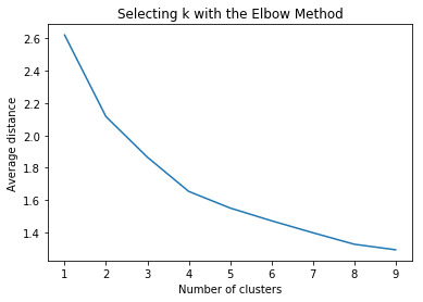
""" Plot average distance from observations from the cluster centroid to use the Elbow Method to identify number of clusters to choose """

plt.plot(clusters, meandist) plt.xlabel('Number of clusters') plt.ylabel('Average distance') plt.title('Selecting k with the Elbow Method')

# Interpret 4 cluster solution model4=KMeans(n_clusters=4) model4.fit(clus_train) clusassign=model4.predict(clus_train) # plot clusters

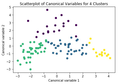
from sklearn.decomposition import PCA pca_2 = PCA(2) plot_columns = pca_2.fit_transform(clus_train) plt.scatter(x=plot_columns[:,0], y=plot_columns[:,1], c=model4.labels_,) plt.xlabel('Canonical variable 1') plt.ylabel('Canonical variable 2') plt.title('Scatterplot of Canonical Variables for 4 Clusters') plt.show()

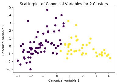
# Interpret 2 cluster solution model2=KMeans(n_clusters=2) model2.fit(clus_train) clusassign=model2.predict(clus_train) # plot clusters

from sklearn.decomposition import PCA pca_2 = PCA(2) plot_columns = pca_2.fit_transform(clus_train) plt.scatter(x=plot_columns[:,0], y=plot_columns[:,1], c=model2.labels_,) plt.xlabel('Canonical variable 1') plt.ylabel('Canonical variable 2') plt.title('Scatterplot of Canonical Variables for 2 Clusters') plt.show()

#We proceed with the 4-cluster model after looking at the plots (attached)

""" BEGIN multiple steps to merge cluster assignment with clustering variables to examine cluster variable means by cluster """ # create a unique identifier variable from the index for the # cluster training data to merge with the cluster assignment variable clus_train.reset_index(level=0, inplace=True) # create a list that has the new index variable cluslist=list(clus_train['index']) # create a list of cluster assignments labels=list(model4.labels_) # combine index variable list with cluster assignment list into a dictionary newlist=dict(zip(cluslist, labels)) newlist # convert newlist dictionary to a dataframe newclus=DataFrame.from_dict(newlist, orient='index') newclus # rename the cluster assignment column newclus.columns = ['cluster']

# now do the same for the cluster assignment variable # create a unique identifier variable from the index for the # cluster assignment dataframe # to merge with cluster training data newclus.reset_index(level=0, inplace=True) # merge the cluster assignment dataframe with the cluster training variable dataframe # by the index variable merged_train=pd.merge(clus_train, newclus, on='index') merged_train.head(n=100) # cluster frequencies merged_train.cluster.value_counts()

""" END multiple steps to merge cluster assignment with clustering variables to examine cluster variable means by cluster """

# FINALLY calculate clustering variable means by cluster clustergrp = merged_train.groupby('cluster').mean() print ("Clustering variable means by cluster") print(clustergrp)

# validate clusters in training data by examining cluster differences in GPA using ANOVA # first have to merge SUICIDEPER100TH with clustering variables and cluster assignment data suicide_data=data_clean['SUICIDEPER100TH'] # split suicide data into train and test sets suicide_train, suicide_test = train_test_split(suicide_data, test_size=.3, random_state=123) suicide_train1=pd.DataFrame(suicide_train) suicide_train1.reset_index(level=0, inplace=True) merged_train_all=pd.merge(suicide_train1, merged_train, on='index')

#sub1 = merged_train_all[['SUICIDEPER100TH', 'cluster']].dropna() sub1 = merged_train_all[['SUICIDEPER100TH', 'cluster']].dropna()

import statsmodels.formula.api as smf import statsmodels.stats.multicomp as multi

suicidemod = smf.ols(formula='SUICIDEPER100TH ~ C(cluster)', data=sub1).fit() print (suicidemod.summary())

print ('means for suicide by cluster') m1= sub1.groupby('cluster').mean() print (m1)

print ('standard deviations for suicide by cluster') m2= sub1.groupby('cluster').std() print (m2)

mc1 = multi.MultiComparison(sub1['SUICIDEPER100TH'], sub1['cluster']) res1 = mc1.tukeyhsd() print(res1.summary())

#############Code End#################

Results:

Clustering variable means by cluster index INCOMEPERPERSON ... LIFEEXPECTANCY URBANRATE cluster ... 0 89.888889 -0.240612 ... 0.227263 0.135969 1 67.942857 -0.228249 ... 0.475045 0.395141 2 82.750000 -0.611545 ... -1.098212 -0.883506 3 76.000000 1.923554 ... 1.159696 0.871168

print (suicidemod.summary()) OLS Regression Results ============================================================================== Dep. Variable: SUICIDEPER100TH R-squared: 0.063 Model: OLS Adj. R-squared: 0.036 Method: Least Squares F-statistic: 2.315 Date: Sun, 24 Mar 2019 Prob (F-statistic): 0.0802 Time: 12:24:10 Log-Likelihood: -342.48 No. Observations: 107 AIC: 693.0 Df Residuals: 103 BIC: 703.6 Df Model: 3 Covariance Type: nonrobust =================================================================================== coef std err t P>|t| [0.025 0.975] ----------------------------------------------------------------------------------- Intercept 6.5936 1.427 4.620 0.000 3.763 9.424 C(cluster)[T.1] 4.3384 1.756 2.470 0.015 0.856 7.821 C(cluster)[T.2] 3.3438 1.718 1.946 0.054 -0.064 6.752 C(cluster)[T.3] 4.5218 2.158 2.096 0.039 0.243 8.801 ============================================================================== Omnibus: 34.985 Durbin-Watson: 2.146 Prob(Omnibus): 0.000 Jarque-Bera (JB): 66.414 Skew: 1.358 Prob(JB): 3.79e-15 Kurtosis: 5.742 Cond. No. 5.93 ==============================================================================

Warnings: [1] Standard Errors assume that the covariance matrix of the errors is correctly specified.

print ('means for suicide by cluster') m1= sub1.groupby('cluster').mean() print (m1) means for suicide by cluster SUICIDEPER100TH cluster 0 6.593638 1 10.932016 2 9.937488 3 11.115407

print ('standard deviations for suicide by cluster') m2= sub1.groupby('cluster').std() print (m2) standard deviations for suicide by cluster SUICIDEPER100TH cluster 0 6.835408 1 8.263957 2 3.310233 3 4.226248

mc1 = multi.MultiComparison(sub1['SUICIDEPER100TH'], sub1['cluster']) res1 = mc1.tukeyhsd() print(res1.summary()) Multiple Comparison of Means - Tukey HSD,FWER=0.05 ============================================= group1 group2 meandiff lower upper reject --------------------------------------------- 0 1 4.3384 -0.2479 8.9247 False 0 2 3.3438 -1.144 7.8317 False 0 3 4.5218 -1.1129 10.1565 False 1 2 -0.9945 -4.6544 2.6653 False 1 3 0.1834 -4.8169 5.1837 False 2 3 1.1779 -3.7323 6.0881 False ---------------------------------------------

Interpretation: A k-means clustering algorithm was run as explained. Using the elbow curve method we used a four cluster solution to interpret and analyse the results. Tukey test was used to compare the mean for the four clusters created and ANOVA was used for comparing the variance.

The results show that both mean and std deviation are significantly different for the suicide rate for the four different clusters.

0 notes

sandeepsrinivas19 · 6 years

Text

House Price Classification - Lasso

House Price Classification

The objective is to classify the price of a house with the given parameters as 0(Price <$500,000) and 1(Price>=$500000) and identify the various parameters responsible for the pricing. The data is for various parameters (predictors) like number of bedrooms, sqft living area, number of bathrooms, whether the house has a view or not etc (from online source) is fed into the classification regression model. Target variable is the price_class of the house.

Code #########################

os.chdir("A:\ML Coursera") #Load the dataset data = pd.read_csv("home_data3.csv")

#upper-case all DataFrame column names data.columns = map(str.upper, data.columns)

# Data Management data_clean = data.dropna()

target = data_clean.PRICE_CLASS

predictors.head() # split data into train and test sets pred_train, pred_test, tar_train, tar_test = train_test_split(predictors, target, test_size=.3, random_state=123)

# specify the lasso regression model model=LassoLarsCV(cv=10, precompute=False).fit(pred_train,tar_train)

# print variable names and regression coefficients dict(zip(predictors.columns, model.coef_))

#########################

Output:

{'BEDROOMS': -0.00042543529151601797, 'BATHROOMS': 0.02735333928831517, 'SQFT_LIVING': 0.08572220222236561, 'SQFT_LOT': 0.007998695399789518, 'FLOORS': 0.04744203874354188, 'WATERFRONT': 0.0015738192746130087, 'VIEW': 0.0171052057946378, 'CONDITION': 0.022601962456814437, 'GRADE': 0.22293970415978565, 'SQFT_ABOVE': 0.0, 'SQFT_BASEMENT': 0.014998665998908652, 'YR_BUILT': -0.14130408055369761, 'YR_RENOVATED': -0.003021277379032161}

training data MSE 0.14746511823540823 test data MSE 0.14729803797546054 training data R-square 0.39345776492926426 test data R-square 0.39651086088327553

The test R-square value is around 40%, which is quite low.

0 notes

sandeepsrinivas19 · 6 years

Text

Random Forest - House Price Classification

The objective is to classify the price of a house with the given parameters as Low (Price <$500,000) and High (Price>=$500000) and identify the various parameters responsible for the pricing. The data is for various parameters (predictors) like number of bedrooms, sqft living area, number of bathrooms, whether the house has a view or not etc (from online source) is fed into the random forest algorithm. Target variable is the price_class of the house.

Code #########################

from pandas import Series, DataFrame import pandas as pd import numpy as np import os import matplotlib.pylab as plt from sklearn.cross_validation import train_test_split from sklearn.tree import DecisionTreeClassifier from sklearn.metrics import classification_report import sklearn.metrics # Feature Importance from sklearn import datasets from sklearn.ensemble import ExtraTreesClassifier

os.chdir("A:\ML Coursera")

#Load the dataset

AH_data = pd.read_csv("home_data2.csv") data_clean = AH_data.dropna()

data_clean.dtypes data_clean.describe()

#Split into training and testing sets

predictors = data_clean[['bedrooms', 'bathrooms', 'sqft_living', 'sqft_lot', 'floors', 'waterfront', 'view' , 'sqft_above', 'sqft_basement', 'yr_built']]

targets = data_clean.price_class targets.head()

pred_train, pred_test, tar_train, tar_test = train_test_split(predictors, targets, test_size=.3)

pred_train.shape pred_test.shape tar_train.shape tar_test.shape

#Build model on training data from sklearn.ensemble import RandomForestClassifier

classifier=RandomForestClassifier(n_estimators=10) classifier=classifier.fit(pred_train,tar_train)

predictions=classifier.predict(pred_test)

sklearn.metrics.confusion_matrix(tar_test,predictions) sklearn.metrics.accuracy_score(tar_test, predictions)

# fit an Extra Trees model to the data model = ExtraTreesClassifier() model.fit(pred_train,tar_train) # display the relative importance of each attribute print(model.feature_importances_)

""" Running a different number of trees and see the effect of that on the accuracy of the prediction """

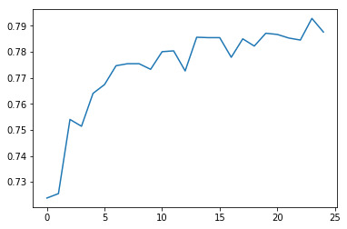
trees=range(25) accuracy=np.zeros(25)

for idx in range(len(trees)): classifier=RandomForestClassifier(n_estimators=idx + 1) classifier=classifier.fit(pred_train,tar_train) predictions=classifier.predict(pred_test) accuracy[idx]=sklearn.metrics.accuracy_score(tar_test, predictions)

plt.cla() plt.plot(trees, accuracy)

###############

Output Summary:

Accuracy: 0.7830043183220234

Feature OOB Gini 'bedrooms', 0.05573633 'bathrooms', 0.08098398 'sqft_living', 0.20783781 'sqft_lot', 0.14737421 'floors', 0.04302802 'waterfront', 0.00146581 'view' 0.0441065 'sqft_above', 0.18545935 'sqft_basement', 0.0822214 'yr_built' 0.15178659

sklearn.metrics.confusion_matrix(tar_test,predictions) array([[2045, 702], [ 659, 3078]], dtype=int64)

The accuracy of predictions as per the matrix is 79%.

0 notes

sandeepsrinivas19 · 6 years

Text

House Price Classification

The objective is to classify the price of a house with the given parameters as Low (Price <$500,000)

and High (Price>=$500000).

The data is for various parameters (predictors) like number of bedrooms, sqft living area, number of bathrooms, whether the house has a view or not etc

(from online source) is fed into the decision tree.

Target variable is the price_class of the house.

#Code

###############################

from pandas import Series, DataFrame

import pandas as pd

import numpy as np

import os

import matplotlib.pylab as plt

from sklearn.cross_validation import train_test_split

from sklearn.tree import DecisionTreeClassifier

from sklearn.metrics import classification_report

import sklearn.metrics

import pydotplus

os.chdir("A:\ML Coursera")

#Load the dataset

home_data = pd.read_csv("home_data2.csv")

data_clean = home_data.dropna()

"""

Modeling and Prediction

"""

#Split into training and testing sets

predictors = data_clean[['bedrooms', 'bathrooms',

'sqft_living', 'sqft_lot', 'floors', 'waterfront'

, 'view', 'sqft_above', 'sqft_basement', 'yr_built']]

targets = data_clean.price_class

targets.shape

pred_train, pred_test, tar_train, tar_test = train_test_split(predictors, targets, test_size=.4)

#Build model on training data

classifier=DecisionTreeClassifier()

classifier=classifier.fit(pred_train,tar_train)

predictions=classifier.predict(pred_test)

sklearn.metrics.confusion_matrix(tar_test,predictions)

sklearn.metrics.accuracy_score(tar_test, predictions)

#Displaying the decision tree

from sklearn import tree

#from StringIO import StringIO

from io import StringIO

#from StringIO import StringIO

from IPython.display import Image

out = StringIO()

tree.export_graphviz(classifier, out_file=out)

out = StringIO()

tree.export_graphviz(classifier, out_file=dotfile)

pydotplus.graph_from_dot_data(out.getvalue()).write_png(“dtree1.png”)

graph=pydotplus.graph_from_dot_data(out.getvalue())

Image(graph.create_png())

from IPython.display import Image

Image(filename = 'tree_limited.png')

#################################

Output:

Confusion Matrix:

array([[2511, 1174],

[1230, 3731]], dtype=int64)

sklearn.metrics.accuracy_score(tar_test, predictions)

Out[8]: 0.7219523479065464

This shows that the accuracy of classification is 72%, which is pretty decent.

Summary:

Hence, the model was able to predict whether the house is low-priced or high-priced with an accuracy of 72%. An improvement in accuracy can be aimed for

if we try to add more variables related to the same to the dataset and observe how they influence the model.

0 notes