rawshunnn

[rawshunnn]

K-Mean Cluster Mean

A k-means cluster analysis was conducted to identify underlying subgroups of adolescents based on their similarity of responses on 11 variables that represent characteristics that could have an impact on school achievement. Clustering variables included two binary variables measuring whether or not the adolescent had ever used alcohol or marijuana, as well as quantitative variables measuring alcohol problems, a scale measuring engaging in deviant behaviors (such as vandalism, other property damage, lying, stealing, running away, driving without permission, selling drugs, and skipping school), and scales measuring violence, depression, self-esteem, parental presence, parental activities, family connectedness, and school connectedness. All clustering variables were standardized to have a mean of 0 and a standard deviation of 1.

Data were randomly split into a training set that included 70% of the observations (N=3201) and a test set that included 30% of the observations (N=1701). A series of k-means cluster analyses were conducted on the training data specifying k=1-9 clusters, using Euclidean distance. The variance in the clustering variables that was accounted for by the clusters (r-square) was plotted for each of the nine cluster solutions in an elbow curve to provide guidance for choosing the number of clusters to interpret.

Code:

# -*- coding: utf-8 -*- """ Created on Mon Jan 18 19:51:29 2016

@author: jrose01 """

from pandas import Series, DataFrame import pandas as pd import numpy as np import matplotlib.pylab as plt from sklearn.model_selection import train_test_split from sklearn import preprocessing from sklearn.cluster import KMeans

""" Data Management """ data = pd.read_csv("tree_addhealth.csv")

#upper-case all DataFrame column names data.columns = map(str.upper, data.columns)

# Data Management

data_clean = data.dropna()

# subset clustering variables cluster=data_clean[['ALCEVR1','MAREVER1','ALCPROBS1','DEVIANT1','VIOL1', 'DEP1','ESTEEM1','SCHCONN1','PARACTV', 'PARPRES','FAMCONCT']] cluster.describe()

# standardize clustering variables to have mean=0 and sd=1 clustervar=cluster.copy() clustervar['ALCEVR1']=preprocessing.scale(clustervar['ALCEVR1'].astype('float64')) clustervar['ALCPROBS1']=preprocessing.scale(clustervar['ALCPROBS1'].astype('float64')) clustervar['MAREVER1']=preprocessing.scale(clustervar['MAREVER1'].astype('float64')) clustervar['DEP1']=preprocessing.scale(clustervar['DEP1'].astype('float64')) clustervar['ESTEEM1']=preprocessing.scale(clustervar['ESTEEM1'].astype('float64')) clustervar['VIOL1']=preprocessing.scale(clustervar['VIOL1'].astype('float64')) clustervar['DEVIANT1']=preprocessing.scale(clustervar['DEVIANT1'].astype('float64')) clustervar['FAMCONCT']=preprocessing.scale(clustervar['FAMCONCT'].astype('float64')) clustervar['SCHCONN1']=preprocessing.scale(clustervar['SCHCONN1'].astype('float64')) clustervar['PARACTV']=preprocessing.scale(clustervar['PARACTV'].astype('float64')) clustervar['PARPRES']=preprocessing.scale(clustervar['PARPRES'].astype('float64'))

# split data into train and test sets clus_train, clus_test = train_test_split(clustervar, test_size=.3, random_state=123)

# k-means cluster analysis for 1-9 clusters                                                           from scipy.spatial.distance import cdist clusters=range(1,10) meandist=[]

for k in clusters:    model=KMeans(n_clusters=k)    model.fit(clus_train)    clusassign=model.predict(clus_train)    meandist.append(sum(np.min(cdist(clus_train, model.cluster_centers_, 'euclidean'), axis=1))    / clus_train.shape[0])

""" Plot average distance from observations from the cluster centroid to use the Elbow Method to identify number of clusters to choose """

plt.plot(clusters, meandist) plt.xlabel('Number of clusters') plt.ylabel('Average distance') plt.title('Selecting k with the Elbow Method')

# Interpret 3 cluster solution model3=KMeans(n_clusters=3) model3.fit(clus_train) clusassign=model3.predict(clus_train) # plot clusters

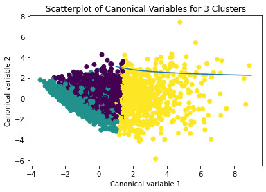
from sklearn.decomposition import PCA pca_2 = PCA(2) plot_columns = pca_2.fit_transform(clus_train) plt.scatter(x=plot_columns[:,0], y=plot_columns[:,1], c=model3.labels_,) plt.xlabel('Canonical variable 1') plt.ylabel('Canonical variable 2') plt.title('Scatterplot of Canonical Variables for 3 Clusters') plt.show()

""" BEGIN multiple steps to merge cluster assignment with clustering variables to examine cluster variable means by cluster """ # create a unique identifier variable from the index for the # cluster training data to merge with the cluster assignment variable clus_train.reset_index(level=0, inplace=True) # create a list that has the new index variable cluslist=list(clus_train['index']) # create a list of cluster assignments labels=list(model3.labels_) # combine index variable list with cluster assignment list into a dictionary newlist=dict(zip(cluslist, labels)) newlist # convert newlist dictionary to a dataframe newclus=DataFrame.from_dict(newlist, orient='index') newclus # rename the cluster assignment column newclus.columns = ['cluster']

# now do the same for the cluster assignment variable # create a unique identifier variable from the index for the # cluster assignment dataframe # to merge with cluster training data newclus.reset_index(level=0, inplace=True) # merge the cluster assignment dataframe with the cluster training variable dataframe # by the index variable merged_train=pd.merge(clus_train, newclus, on='index') merged_train.head(n=100) # cluster frequencies merged_train.cluster.value_counts()

""" END multiple steps to merge cluster assignment with clustering variables to examine cluster variable means by cluster """

# FINALLY calculate clustering variable means by cluster clustergrp = merged_train.groupby('cluster').mean() print ("Clustering variable means by cluster") print(clustergrp)

# validate clusters in training data by examining cluster differences in GPA using ANOVA # first have to merge GPA with clustering variables and cluster assignment data gpa_data=data_clean['GPA1'] # split GPA data into train and test sets gpa_train, gpa_test = train_test_split(gpa_data, test_size=.3, random_state=123) gpa_train1=pd.DataFrame(gpa_train) gpa_train1.reset_index(level=0, inplace=True) merged_train_all=pd.merge(gpa_train1, merged_train, on='index') sub1 = merged_train_all[['GPA1', 'cluster']].dropna()

import statsmodels.formula.api as smf import statsmodels.stats.multicomp as multi

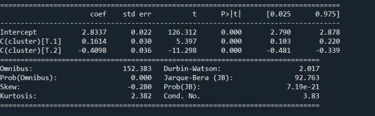
gpamod = smf.ols(formula='GPA1 ~ C(cluster)', data=sub1).fit() print (gpamod.summary())

print ('means for GPA by cluster') m1= sub1.groupby('cluster').mean() print (m1)

print ('standard deviations for GPA by cluster') m2= sub1.groupby('cluster').std() print (m2)

mc1 = multi.MultiComparison(sub1['GPA1'], sub1['cluster']) res1 = mc1.tukeyhsd() print(res1.summary())

Solution:

Conclusion:

The Graph shows the observations are divided into 3 groups on the basis of the residual distance. The analysis was successful using K mean cluster.

[rawshunnn]

Lasso Regression

A lasso regression analysis was conducted to identify a subset of variables from a pool of 23 categorical and quantitative predictor variables that best predicted a quantitative response variable measuring school connectedness in adolescents. Categorical predictors included gender and a series of 5 binary categorical variables for race and ethnicity (Hispanic, White, Black, Native American and Asian) to improve interpret ability of the selected model with fewer predictors. Binary substance use variables were measured with individual questions about whether the adolescent had ever used alcohol, marijuana, cocaine or inhalants. Additional categorical variables included the availability of cigarettes in the home, whether or not either parent was on public assistance and any experience with being expelled from school. Quantitative predictor variables include age, alcohol problems, and a measure of deviance that included such behaviors as vandalism, other property damage, lying, stealing, running away, driving without permission, selling drugs, and skipping school. Another scale for violence, one for depression, and others measuring self-esteem, parental presence, parental activities, family connectedness and grade point average were also included. All predictor variables were standardized to have a mean of zero and a standard deviation of one.

Code:

# -*- coding: utf-8 -*- """ Created on Mon Dec 14 16:26:46 2015

@author: jrose01 """

#from pandas import Series, DataFrame import pandas as pd import numpy as np import matplotlib.pylab as plt from sklearn.model_selection import train_test_split from sklearn.linear_model import LassoLarsCV

#Load the dataset data = pd.read_csv("tree_addhealth.csv")

#upper-case all DataFrame column names data.columns = map(str.upper, data.columns)

# Data Management data_clean = data.dropna() recode1 = {1:1, 2:0} data_clean['MALE']= data_clean['BIO_SEX'].map(recode1)

#select predictor variables and target variable as separate data sets   predvar= data_clean[['MALE','HISPANIC','WHITE','BLACK','NAMERICAN','ASIAN', 'AGE','ALCEVR1','ALCPROBS1','MAREVER1','COCEVER1','INHEVER1','CIGAVAIL','DEP1', 'ESTEEM1','VIOL1','PASSIST','DEVIANT1','GPA1','EXPEL1','FAMCONCT','PARACTV', 'PARPRES']]

target = data_clean.SCHCONN1

# standardize predictors to have mean=0 and sd=1 predictors=predvar.copy() from sklearn import preprocessing predictors['MALE']=preprocessing.scale(predictors['MALE'].astype('float64')) predictors['HISPANIC']=preprocessing.scale(predictors['HISPANIC'].astype('float64')) predictors['WHITE']=preprocessing.scale(predictors['WHITE'].astype('float64')) predictors['NAMERICAN']=preprocessing.scale(predictors['NAMERICAN'].astype('float64')) predictors['ASIAN']=preprocessing.scale(predictors['ASIAN'].astype('float64')) predictors['AGE']=preprocessing.scale(predictors['AGE'].astype('float64')) predictors['ALCEVR1']=preprocessing.scale(predictors['ALCEVR1'].astype('float64')) predictors['ALCPROBS1']=preprocessing.scale(predictors['ALCPROBS1'].astype('float64')) predictors['MAREVER1']=preprocessing.scale(predictors['MAREVER1'].astype('float64')) predictors['COCEVER1']=preprocessing.scale(predictors['COCEVER1'].astype('float64')) predictors['INHEVER1']=preprocessing.scale(predictors['INHEVER1'].astype('float64')) predictors['CIGAVAIL']=preprocessing.scale(predictors['CIGAVAIL'].astype('float64')) predictors['DEP1']=preprocessing.scale(predictors['DEP1'].astype('float64')) predictors['ESTEEM1']=preprocessing.scale(predictors['ESTEEM1'].astype('float64')) predictors['VIOL1']=preprocessing.scale(predictors['VIOL1'].astype('float64')) predictors['PASSIST']=preprocessing.scale(predictors['PASSIST'].astype('float64')) predictors['DEVIANT1']=preprocessing.scale(predictors['DEVIANT1'].astype('float64')) predictors['GPA1']=preprocessing.scale(predictors['GPA1'].astype('float64')) predictors['EXPEL1']=preprocessing.scale(predictors['EXPEL1'].astype('float64')) predictors['FAMCONCT']=preprocessing.scale(predictors['FAMCONCT'].astype('float64')) predictors['PARACTV']=preprocessing.scale(predictors['PARACTV'].astype('float64')) predictors['PARPRES']=preprocessing.scale(predictors['PARPRES'].astype('float64'))

# split data into train and test sets pred_train, pred_test, tar_train, tar_test = train_test_split(predictors, target,                                                              test_size=.3, random_state=123)

# specify the lasso regression model model=LassoLarsCV(cv=10, precompute=False).fit(pred_train,tar_train)

# print variable names and regression coefficients dict(zip(predictors.columns, model.coef_))

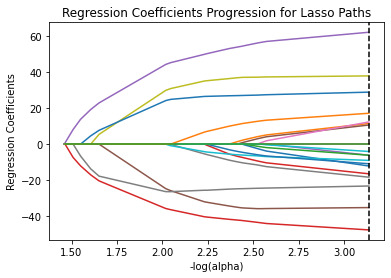
# plot coefficient progression m_log_alphas = -np.log10(model.alphas_) ax = plt.gca() plt.plot(m_log_alphas, model.coef_path_.T) plt.axvline(-np.log10(model.alpha_), linestyle='--', color='k',            label='alpha CV') plt.ylabel('Regression Coefficients') plt.xlabel('-log(alpha)') plt.title('Regression Coefficients Progression for Lasso Paths')

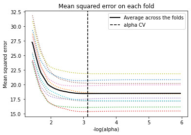
# plot mean square error for each fold m_log_alphascv = -np.log10(model.cv_alphas_) plt.figure() plt.plot(m_log_alphascv, model.mse_path_, ':') plt.plot(m_log_alphascv, model.mse_path_.mean(axis=-1), 'k',         label='Average across the folds', linewidth=2) plt.axvline(-np.log10(model.alpha_), linestyle='--', color='k',            label='alpha CV') plt.legend() plt.xlabel('-log(alpha)') plt.ylabel('Mean squared error') plt.title('Mean squared error on each fold')

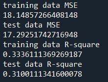
# MSE from training and test data from sklearn.metrics import mean_squared_error train_error = mean_squared_error(tar_train, model.predict(pred_train)) test_error = mean_squared_error(tar_test, model.predict(pred_test)) print ('training data MSE') print(train_error) print ('test data MSE') print(test_error)

# R-square from training and test data rsquared_train=model.score(pred_train,tar_train) rsquared_test=model.score(pred_test,tar_test) print ('training data R-square') print(rsquared_train) print ('test data R-square') print(rsquared_test)

Output:

Conclusion:

Of the 23 predictor variables, 18 were retained in the selected model. During the estimation process, self-esteem and depression were most strongly associated with school connectedness, followed by engaging in violent behavior and GPA. Depression and violent behavior were negatively associated with school connectedness and self-esteem and GPA were positively associated with school connectedness. Other predictors associated with greater school connectedness included older age, Hispanic and Asian ethnicity, family connectedness, and parental involvement in activities. Other predictors associated with lower school connectedness included being male, Black and Native American ethnicity, alcohol, marijuana, and cocaine use, availability of cigarettes at home, deviant behavior, and history of being expelled from school. These 18 variables accounted for 33.4% of the variance in the school connectedness response variable.

[rawshunnn]

Random Forrest

Code:

from pandas import Series, DataFrame import pandas as pd import numpy as np import os import matplotlib.pylab as plt from sklearn.model_selection

import train_test_split from sklearn.tree import DecisionTreeClassifier from sklearn.metrics import classification_report import sklearn.metrics # Feature Importance from sklearn import datasets from sklearn.ensemble import ExtraTreesClassifier

#Load the dataset

AH_data = pd.read_csv("tree_addhealth.csv") data_clean = AH_data.dropna()

data_clean.dtypes data_clean.describe()

#Split into training and testing sets

predictors = data_clean[['BIO_SEX','HISPANIC','WHITE','BLACK','NAMERICAN','ASIAN','age','ALCEVR1','ALCPROBS1','marever1','cocever1','inhever1','cigavail','DEP1','ESTEEM1','VIOL1', 'PASSIST','DEVIANT1','SCHCONN1','GPA1','EXPEL1','FAMCONCT','PARACTV','PARPRES']]

targets = data_clean.TREG1

pred_train, pred_test, tar_train, tar_test  = train_test_split(predictors, targets, test_size=.4)

pred_train.shape pred_test.shape tar_train.shape tar_test.shape

#Build model on training data from sklearn.ensemble import RandomForestClassifier

classifier=RandomForestClassifier(n_estimators=25) classifier=classifier.fit(pred_train,tar_train)

predictions=classifier.predict(pred_test)

sklearn.metrics.confusion_matrix(tar_test,predictions) sklearn.metrics.accuracy_score(tar_test, predictions)

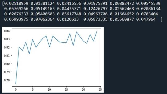
# fit an Extra Trees model to the data model = ExtraTreesClassifier() model.fit(pred_train,tar_train) # display the relative importance of each attribute print(model.feature_importances_)

""" Running a different number of trees and see the effect of that on the accuracy of the prediction """

trees=range(25) accuracy=np.zeros(25)

for idx in range(len(trees)):   classifier=RandomForestClassifier(n_estimators=idx + 1)   classifier=classifier.fit(pred_train,tar_train)   predictions=classifier.predict(pred_test)   accuracy[idx]=sklearn.metrics.accuracy_score(tar_test, predictions)

plt.cla() plt.plot(trees, accuracy)

Output:

Summary/Conclusion:

The research question is about which criteria that affect smoking. I have considered all the explanatory variable but as per the output you can see that marijuana consumption is the factor that contributes the most in regular smoking, where as some factors have very less influence such as GPA or expulsion from school, this helps us make a better and a more informed decision about which factors must be considered while making the decision tress and which factors don’t affect the decision tree.

[rawshunnn]

Decision Tree

The Decision Tree.

now,

Code:

from pandas import Series, DataFrame import pandas as pd import numpy as np import os import matplotlib.pylab as plt from sklearn.model_selection import train_test_split from sklearn.tree import DecisionTreeClassifier from sklearn.metrics import classification_report import sklearn.metrics

os.chdir("D:\Working Directory")

""" Data Engineering and Analysis """ #Load the dataset

AH_data = pd.read_csv("tree_addhealth.csv")

data_clean = AH_data.dropna()

data_clean.dtypes data_clean.describe()

""" Modeling and Prediction """ #Split into training and testing sets

predictors = data_clean[['ALCEVR1','marever1']]

targets = data_clean.TREG1

pred_train, pred_test, tar_train, tar_test  =   train_test_split(predictors, targets, test_size=.4)

pred_train.shape pred_test.shape tar_train.shape tar_test.shape

#Build model on training data classifier=DecisionTreeClassifier() classifier=classifier.fit(pred_train,tar_train)

predictions=classifier.predict(pred_test)

a=sklearn.metrics.confusion_matrix(tar_test,predictions) b=sklearn.metrics.accuracy_score(tar_test, predictions)

print(a) print(b)

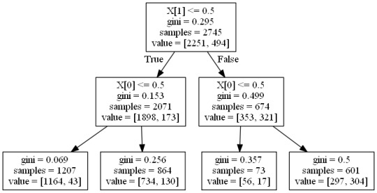
#Displaying the decision tree from sklearn import tree #from StringIO import StringIO from io import StringIO #from StringIO import StringIO from IPython.display import Image out = StringIO() tree.export_graphviz(classifier, out_file=out) import pydotplus graph=pydotplus.graph_from_dot_data(out.getvalue()) c=Image(graph.create_png()) display(c)

Output:

The Confusion matrix and the accuracy score is:

Summary:

According to the output we get 195 false positives and 137 false negatives, whereas we get 1322 and 195 True Positives and True Negatives Respectively.The accuracy score is 0.81. The test accuracy is set at 60% while sample accuracy is set 40%.In the decision tree first differentiator is alcohol consumption and then it marijuana intake. First we get 2251 people who drink alcohol out of which 1898 take marijuana and from that group we see 1164 who addicted to smoking similarly in other group the results and impact of predictors on target.

[rawshunnn]

Logistic Regression

Research Question:

Is alcohol consumption of a country related to the urban rate of the country? Also I have taken into consideration the employment rate of the country  as a co-founding variable.

The dataset used is gapminder, but since all the data in the data set are quantitative variable, I converted alcohol consumption into 2 groups and employment rate into 3 groups.

Code:

import numpy import pandas as pd import statsmodels.formula.api as smf

# bug fix for display formats to avoid run time errors pd.set_option('display.float_format', lambda x:'%.2f'%x)

#To display all the rows and columns pd.set_option('display.max_columns',None) pd.set_option('display.max_rows',None)

#Importing the dataset data=pd.read_csv('gapminder.csv',low_memory=False)

#To avoid runtime errors pd.set_option('display.float_format',lambda x:'%f'%x)

#Converting all the required data to float data['alcconsumption']=pd.to_numeric(data['alcconsumption'], errors='coerce').fillna(99) data['lifeexpectancy']=pd.to_numeric(data['lifeexpectancy'],errors='coerce').fillna(0) data['incomeperperson']=pd.to_numeric(data['incomeperperson'],errors='coerce').fillna(0) data['employrate']=pd.to_numeric(data['employrate'],errors='coerce').fillna(0) data['urbanrate']=pd.to_numeric(data['urbanrate'],errors='coerce').fillna(0)

#converting all missing values to nan data['alcconsumption']=data['alcconsumption'].replace(99,numpy.nan) data['urbanrate']=data['urbanrate'].replace(0,numpy.nan) data['employrate']=data['employrate'].replace(0,numpy.nan)

sub=data[['alcconsumption','urbanrate','employrate']] sub1=sub.copy().dropna()

sub1['alcogrp']=pd.qcut(sub1.alcconsumption,2,['0','1']) sub1['alcogrp']=pd.to_numeric(sub1['alcogrp'],errors='coerce')

sub1['empgrp']=pd.qcut(sub1.employrate,4,['0','1','2','3']) sub1['empgrp']=pd.to_numeric(sub1['empgrp'],errors='coerce')

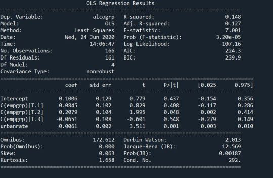
lreg =smf.ols(formula='alcogrp ~ urbanrate + C(empgrp)',data=sub1).fit() print(lreg.summary())

print('\nOdd Ratios') print(numpy.exp(lreg.params))

Output:

Logistic Regression:

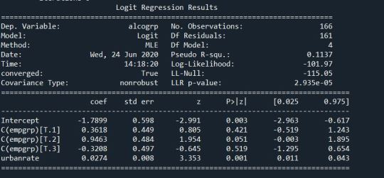
Summary:

According to the regression model and the logistic regression model you can see that urban rate of a country is positively associated to alcohol consumption of a country when the employment rate is controlled. The p-value of urban rate is 0.001 which less than 0.05 and the odd ratios for the same is 1.00 . The association between the alcohol consumption and employment rate however is cannot be seen, when urban rate is controlled.

Association:

There is a positive and weak association between urban rate and alcohol consumption, in presence of employment rate.

[rawshunnn]

Multiple regression

Research Question:

Is alcohol consumption of a country is associated with the urbanization of the country. I have also taken into consideration the average income per person of that country as a co founding variable.

Code:

import numpy import pandas as pd import matplotlib.pyplot as plt import statsmodels.api as sm import statsmodels.formula.api as smf import seaborn

# bug fix for display formats to avoid run time errors pd.set_option('display.float_format', lambda x:'%.2f'%x)

#Importing the dataset data=pd.read_csv('gapminder.csv',low_memory=False)

#To avoid runtime errors pd.set_option('display.float_format',lambda x:'%f'%x)

#Converting all the required data to float data['alcconsumption']=pd.to_numeric(data['alcconsumption'], errors='coerce').fillna(99) data['incomeperperson']=pd.to_numeric(data['incomeperperson'],errors='coerce').fillna(0) data['urbanrate']=pd.to_numeric(data['urbanrate'],errors='coerce').fillna(0)

#copying sub to sub1 to avoid errors sub=data[['urbanrate','alcconsumption','incomeperperson',]] sub1=sub.copy()

#converting all missing values to nan sub1['alcconsumption']=sub1['alcconsumption'].replace(99,numpy.nan) sub1['incomeperperson']=sub1['incomeperperson'].replace(0,numpy.nan) sub1['urbanrate']=sub1['urbanrate'].replace(0,numpy.nan) sub3=sub1.copy() sub4=sub3.dropna() sub2=sub4.copy() #################################################################################### # POLYNOMIAL REGRESSION ####################################################################################

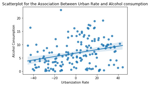
# first order (linear) scatterplot scat1 = seaborn.regplot(x="urbanrate", y="alcconsumption", scatter=True, data=sub2) plt.xlabel('Urbanization Rate') plt.ylabel('Alcohol Consumption Rate')

# fit second order polynomial # run the 2 scatterplots together to get both linear and second order fit lines scat1 = seaborn.regplot(x="urbanrate", y="alcconsumption", scatter=True, order=2, data=sub2) plt.xlabel('Urbanization Rate') plt.ylabel('Alcohol Consumption Rate')

# center quantitative IVs for regression analysis sub2['urbanrate_c'] = (sub2['urbanrate'] - sub2['urbanrate'].mean()) sub2['incomeperperson_c'] = (sub2['incomeperperson'] - sub2['incomeperperson'].mean()) sub2[["urbanrate_c", "incomeperperson_c"]].describe()

# linear regression analysis reg1 = smf.ols('alcconsumption ~ urbanrate_c', data=sub2).fit() print (reg1.summary())

# quadratic (polynomial) regression analysis

# run following line of code if you get PatsyError 'ImaginaryUnit' object is not callable reg2 = smf.ols('alcconsumption ~ urbanrate_c + I(urbanrate_c**2)', data=sub2).fit() print (reg2.summary())

#################################################################################### # EVALUATING MODEL FIT ####################################################################################

# adding internet use rate reg3 = smf.ols('alcconsumption  ~ urbanrate_c + I(urbanrate_c**2) + incomeperperson_c',               data=sub2).fit() print (reg3.summary())

#Q-Q plot for normality fig4=sm.qqplot(reg3.resid, line='r')

# simple plot of residuals stdres=pd.DataFrame(reg3.resid_pearson) plt.plot(stdres, 'o', ls='None') l = plt.axhline(y=0, color='r') plt.ylabel('Standardized Residual') plt.xlabel('Observation Number')

# additional regression diagnostic plots fig2 = plt.figure(figsize=(12,8)) fig2 = sm.graphics.plot_regress_exog(reg3,  "incomeperperson_c", fig=fig2)

# leverage plot fig3=sm.graphics.influence_plot(reg3, size=8) print(fig3)

Regression Model:

Regression Model with only Urban Rate(centered):

Regression model with 1st and 2nd order urban rate (centered) :

Regression model with 1st and 2nd order urban rate (centered)  and Incomeperperson (centered):

Summary:

When we take into consideration only the first order centered urban rate we see that P- value is very small about 0.0001. The intercept is 6.86 and the explanatory coefficient is 0.0595, which means there is an association but the variability is on at 7%. When we add the 2nd Order Centered urban rate we can see the curvilinear graph makes more sense than the linear graph but the variability is around 8% and the p-value for 2nd order urbanrate is high. When we add income per person we get variability of 13% and we get a negative association between 2 order urban rate.

Graph:

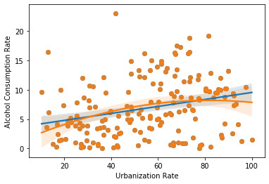
Here you can see curvilinear lines have a better hold on the graph.

QQ-plot:

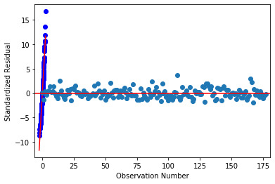
Evaluation of the regression model:

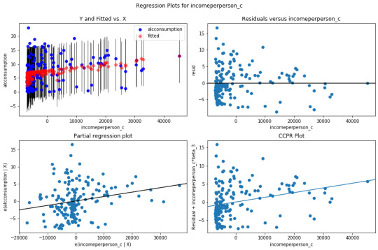
Incomeperperson as a co founding variable has a lot of residuals at lower income group and less at higher income groups.

Leverage Model:

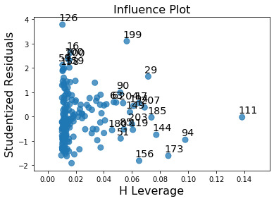
There are residual outliers but they don’t affect the residual model. 

Output:

We can see a weak association between the primary explanatory variable and the response variable, especially in the presence of the co-founding variable. There are outlier but they don’t affect the regression model. The graphs follow the regression assumption. But the proof isn’t enough to say that urbanization has an association with alcohol consumption. 

[rawshunnn]

Basic Linear Regression

Research Question:

Does Alcohol Consumption of country depend on the Urban Rate of the country?

Since the explanatory variable Urban Rate is a quantitative variable it required centering.

Therefore:

Code:

Solution:

Then regression,

Code:

Solution:

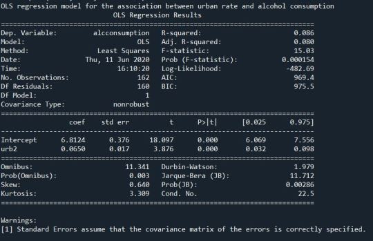
Summary:

The mean before the centering of explanatory variable was 55.82209 and that after centering was very small and close to zero . Then after performing the regression we get the p- value of 0.000154 and F-statistic value of 15.03. The linear regression equation we get is Alcohol Consumption = 6.8124 + 0.065*UrbanRate. The variability will be around 8.6%. We also get a scatter plot graph

[rawshunnn]

Procedures:

The analysis was made to find the relation between the alcohol consumption of a country and the urban rate of that country.

Research Question- Does the alcohol consumption of a country depend upon the urban rate?

The Urban rate was the explanatory variable. Urban population refers to people living in urban areas as defined by national statistical offices (calculated using World Bank population estimates and urban ratios from the United Nations World Urbanization Prospects). The data was given was available in percentage ( % of population living in urban areas)

The alcohol consumption was the response variable. Recorded and estimated average alcohol consumption, adult (15+) per ca-pita consumption in litres pure alcohol. The data was recorded by the WHO.

Both the Data was made available in the year 2008.

Data Management: I removed the unknown data from both the variables. Then I divide both the variables in 5 groups, since both the variables were quantitative variables. 

[rawshunnn]

Measure:

GapMinder collects data from a handful of sources across the globe and made available to us through GapMinder. The data was collected through global-level surveys by organizations such as WHO, International Labor Organization, World Bank and many other such organizations to find out the social, economical and health issue globally. In our analysis we use the the Data Set to find the relation between the urban rate and alcohol consumption of a country. We take into consideration the life expectancy, income per person and employment rate into consideration.

[rawshunnn]

Sample:

The GapMinder Data Set was used for my analysis.GapMinder is a non-profit organization venture promoting global development and achievements of the United Nations Millennium Development Goals. It seeks to increase the use and understanding of statistics about social,economic and environmental development at global level. It was started in the year 2005 and since it’s inception it has grown to include the data of 192 countries that are UN members and additionally includes data for 24 other countries. It includes factors such as the income per person, alcohol consumption, urbanization, life expectancy, employment rate etc. The study was made on a global level. The total observation on the Data Set is 216 countries( 192 UN Members and 24 Others).I included all the countries available in the Data Set.

[rawshunnn]

Writing About Our Data:

Sample:

GapMinder is a non-profit organization venture promoting global development and achievements of the United Nations Millennium Development Goals. It seeks to increase the use and understanding of statistics about social,economic and environmental development at global level. It was started in the year 2005 and since it’s inception it has grown to include the data of 192 countries that are UN members and additionally includes data for 24 other countries. It includes factors such as the income per person, alcohol consumption, urbanization, life expectancy, employment rate etc.

Measure:

GapMinder collects data from a handful of sources, including the Institute for Health Metrics and Evaluation, US Census Bureau’s International Database, United Nations Statistics Division and the World Bank.

Procedure:

All the health related variables such as life expectancy,alcohol consumption, suicide rate in the data set were drawn from the world health organizations country level surveillance and made available to us through gapminder. The variables such as urban rate, income per person, internet usage of a country were drawn from the world bank’s survey. World Labor organisation contributed the data related to employment rate.My analysis was to find a relation between the alcohol consumption(response variable) and the urban rate(expalnatory variable) of a country, here we got the co founding variables such as income per person, employment rate of the countries.

[rawshunnn]

Potential Moderator Test -Statistical Interaction

Moderator test is used to see if a third variable or the moderator variable is associated with the explanatory variable and response variable.

I am using the gapminder data set and therefore I used pearson analysis tool on my data set.

Code: 

Solution:

Graphs:

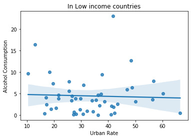
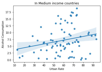
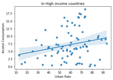
Summary:

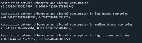
The relation between alcohol consumption and urbanization rate is studied with income group as the moderator. Before the division in income groups. We get the r-value of 0.293 and I divided it in income groups we get r-values -0.04, 0.241 and -0.232 in low, medium and high income groups. The r-value is show the strong or weak linear relation between the two variables. In this case we can see low income group countries have a weak linear relation between alcohol consumption and urbanization. The medium and high income groups have strong linear relation. The graph supports the theory.

[rawshunnn]

Pearson Correlation

Pearson correlation is used when both the variables are quantitative. In my case the two variables are alcohol consumption and urban rate of a country.

Code:

Here I created a new dataset with only the required variables and removed all the unknown variables so that there are no errors during calculations.

The Graph:

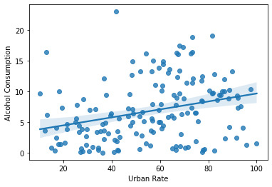
The graph is scatter plot between my two variables and it show a positive linear relation between them. Next we we find the r-value and p-value.

Pearson ‘’r’ value:

Therefore here we get the r-value of 0.29 and a p-value of 0.00015. The r value indicates that the relation is a weak relation . Variability of the relation which is given by the calculation of r^2 is 0.085, therefore the variability is only on 8.5%.

Summary:

We plotted the scatter plot which gave us the relation between the two variables.Then we found out the r value ,p- value and the variability. After all this we can summarize that the urban rate and alcohol consumption have a weak positive linear relation.  

[rawshunnn]

Chi-Squared Test

I am using the gapminder data set to study the relation between alcohol consumption and urban rate of a country. Since all the data in gap minder is in quantitative form. Therefore I’ve have converted the two variables to be compared into categorical variables. 

Alcohol Consumption is divided into 5 groups:

0-5 litres per ca-pita - 1

5.1-10 litres per ca-pita -2

10.1-15 litres per ca-pita-3  

15.1-20 litres per ca-pita -4

20.1-25 litres per ca-pita -5

Urban Consumption is divided into 2 groups:

Urbanization Under 50% - 0

Urbanization Over 50% - 1  

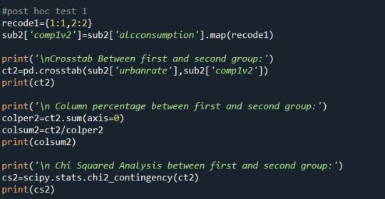
Code 1:

Here after all the initial steps we perform the Chi-Squared Test for the 2 variables.  We print a cross tab between the urban rate and alcohol consumption. Then we get a sum and sum percentage for all the groups. And we do the chi squared test. 

Here we get p-value of 0.00001 and chi square value of 27.77. The p-value is less than 0.05 that means we can ignore the null hypothesis.

We also calculate the Bonferroni Adjustment which is 0.005, which is required for the post HOC test. 

Post HOC test:

Since this isn’t my main analysis I have compared only two groups.Just to test the Chi-Squared Test.

Group 1 and Group 2:

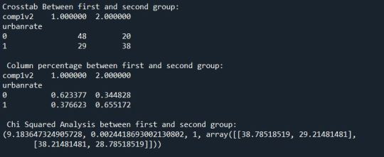
Group 1 and Group 4:

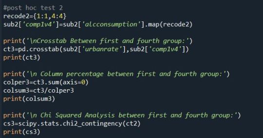
According to the Post HOC test we can ignore the Null Hypothesis. And agree in the Alternate Hypothesis.

Summary:

We can come to a conclusion that we can agree on the alternate analysis since even after the post HOC test we got p-value less than the Bonferroni Adjustment.

[rawshunnn]

Analysis Variance (ANOVA)

ANOVA is a bi-variate statistical tool used to calculate the F-statistics and P- Value when the explanatory variable is categorical and response variable is quantitative. In my analysis I have been using the gapminder data set which consists of only quantitative variables. Therefore I had to convert my explanatory variable into categorical variable. I am studying the effects of alcohol consumption of a country on it’s life expectancy. Therefore my response variable is Life Expectancy and the explanatory variable is alcohol consumption.

The Hypothesis for this study are:

Null Hypothesis- There is no relation between a country’s life expectancy and alcohol consumption per ca pita(in litres)

Alternate Hypothesis- There is a relation between a country’s life expectancy and alcohol consumption per ca pita(in litres)

Dividing Explanatory Variable into categories:

Here the divide the alcohol consumption variable into 4 categories and put them under the variable alcogrp.

Finding the F-Statistics and P-Value:

Code:

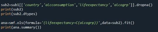
Here we have made a new data set that includes only the required variables. Then used the OLS function under the statsmodels.formula.api library. This will show us the F- Statistics and P-value, so that we can decide if we can ignore the null hypothesis and agree on the the alternate hypothesis.

Output:

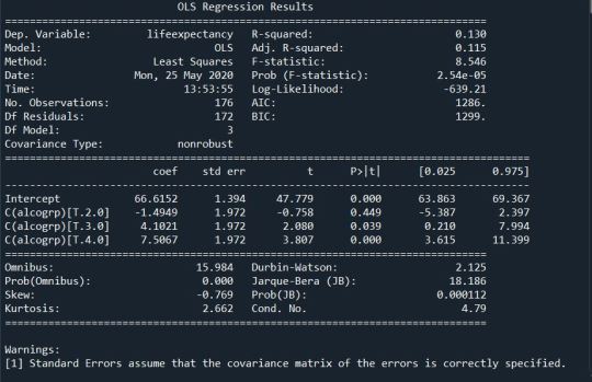
Therefore we get a an F-statistic of 8.546 and the P- Value is 0.00002. There we can justify ignoring the null hypothesis.

POST HOC TEST:

Post HOC test is required to see that we don’t make a wrong decision by ignoring the null hypothesis, or make the type 1 error.

CODE:

Firstly we see the mean and std deviation of the alcogrp.

Then we perform the post hoc test.

Solution:

Here we see after the that after the post hoc test we see we cannot reject the null hypothesis.

Summary:

Therefore,we get the results of ANOVA test.After the OLS function we came to a conclusion that the null hypothesis can be ignored. But on doing Post HOC test we have a different conclusion.

[rawshunnn]

Graphical Representation

I have done plotted three graphs for this data analysis project. Two of which are uni-variate and one is a bi-variate.

The bi-variate graphs show the relation between urbanization and suicide rate.

The urbanization uni variate graph:

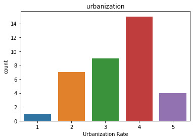
The Graph shows the count of all the countries that have a suicide rate of over 15 person per 100000. Here you can see that most countries allotted to the 4th group are present in this list.

The Suicide Rate uni variate graph:

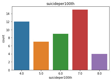
The Suicide Rate are divided into different groups and the frequency is shown.

The Bi Variate Graph:

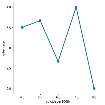
This shows the relation between urbanization and suicide rates. The suicides in the countries in urbanization group 2 have the most suicides i.e the countries that fall under the group that has urbanization in between 20.1-40%, whereas countries that are in group 5(80.1-100%) have the least. But surprisingly the countries that fall in the 3rd group of urbanization have less number of suicides as compared to the countries that fall under the 4th group. This will lead to further analyzing why and what are the factors affecting it. It can be alcohol consumption or employment rates. But according to this survey we see countries that have 100% urbanization don’t see a lot of suicides but the countries that have very little or average urbanization do.

[rawshunnn]

Data Management

Managing data is a very important part of data analysis. I have used the data management technique to find out and replace the data that had no value or no effect on my analysis.

Code:

I have replaced the numeric value 9 which holds the position for unknown value.

Solution:

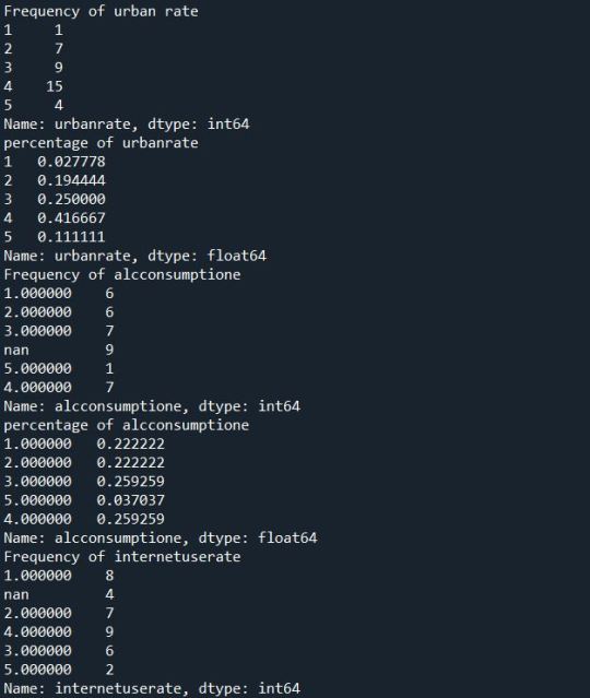
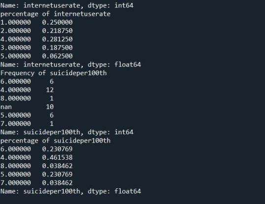
Summary:

After we replace the numeric value 9 with Nan. We find out and display the frequency and percentage distribution of each variable. Here we have considered the countries which are in the 4th group or above of the suicide rate variable. There this data set will exclude the countries where the suicides are less than 15 per 100000. On further Frequency and Percentage distribution we find out that of the countries include most of them fall under the 4th group of urbanization,i.e countries where urbanization rate is between 60-80%. Similarly we have divided other variables that may or may not interfere with our final analysis into detailed frequency and percentage distribution.