rambarad - Tumblr blog

[rambarad]

⚠️ Watch video ⚠️

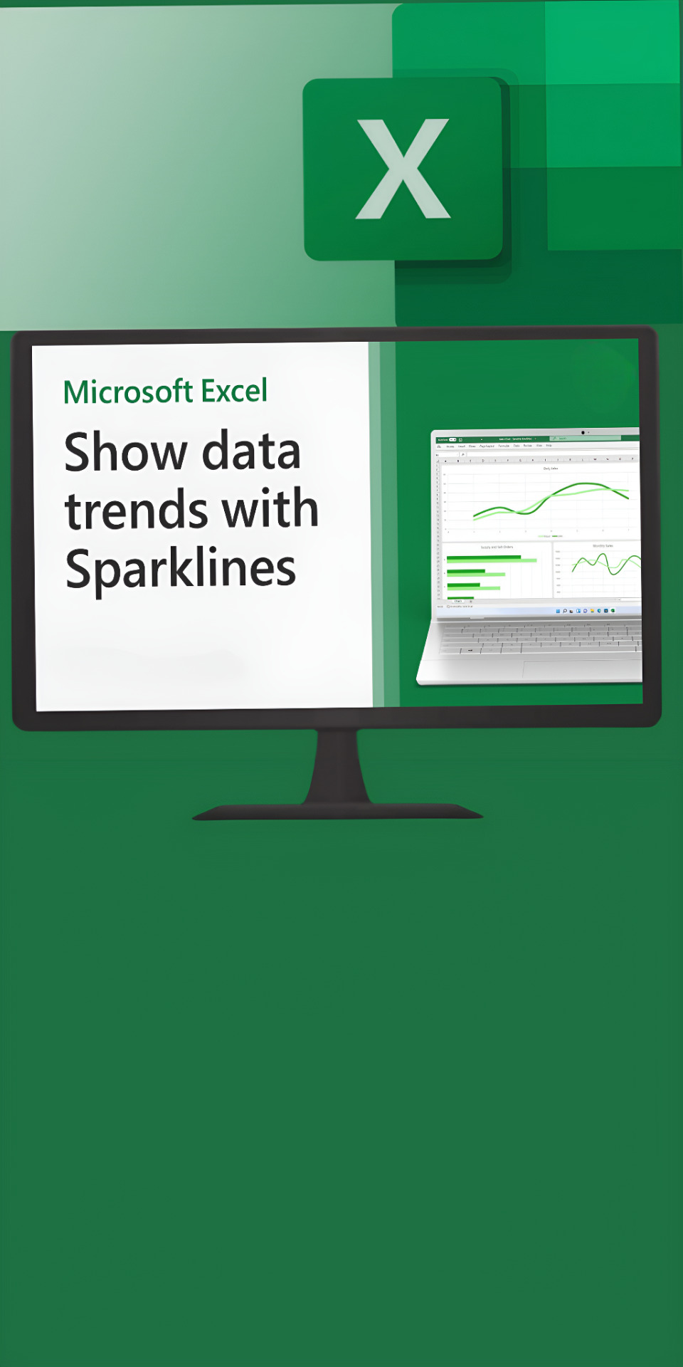
Select the data range for the sparklines.

On the Insert tab, click Sparklines, and then click the kind of sparkline that you want. ...

On the sheet, select the cell or the range of cells where you want to put the sparklines. ...

How to add?

Excel 2016: Click Insert > Insert Column or Bar Chart icon, and select a column chart option of your choice.

Excel 2013: Click Insert > Insert Column Chart icon, and select a column chart option of your choice.

[rambarad]

⚠️Read Caption ⚠️

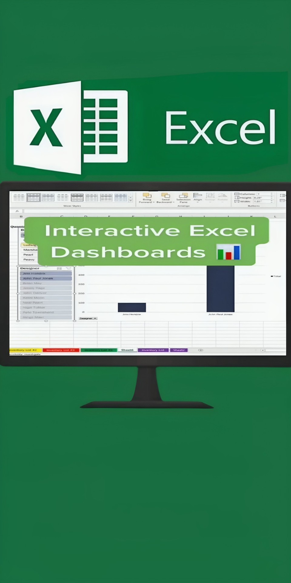
Interactive Excel Dashboard 📊

Customize your dashboard

You can also customize the colors, fonts, typography, and layouts of your charts. 

Additionally, if you wish to make an interactive dashboard, go for a dynamic chart.

A dynamic chart is a regular Excel chart where data updates automatically as you change the data source.

You can bring interactivity using Excel features like:

Macros: automate repetitive actions (you may have to learn Excel VBA for this)

Drop-down lists: allow quick and limited data entry

Slicers: filter data on a Pivot Table

[rambarad]

#excel #exceltutorial #tips

🚀Step by step guide 🚀

^Save this video for future reference^.

VSTACK returns the array formed by appending each of the array arguments in a row-wise fashion. The resulting array will be the following dimensions: Rows: the combined count of all the rows from each of the array arguments. Columns: The maximum of the column count from each of the array arguments.

Syntax

=VSTACK(array1,[array2],...)

The VSTACK function syntax has the following argument:

array The arrays to append.

Remarks

VSTACK returns the array formed by appending each of the array arguments in a row-wise fashion. The resulting array will be the following dimensions:

Rows: the combined count of all the rows from each of the array arguments.

Columns: The maximum of the column count from each of the array arguments.

Errors

If an array has fewer columns than the maximum width of the selected arrays, Excel returns a #N/A error in the additional columns. Use VSTACK inside the IFERROR function to replace #N/A with the value of your choice.

[rambarad]

The XLOOKUP function to find things in a table or range by row. For example, look up the price of an automotive part by the part number, or find an employee name based on their employee ID. With XLOOKUP, you can look in one column for a search term and return a result from the same row in another column, regardless of which side the return column is on.

Note: XLOOKUP is not available in Excel 2016 and Excel 2019, however, you may come across a situation of using a workbook in Excel 2016 or Excel 2019 with the XLOOKUP function in it created by someone else using a newer version of Excel.

Syntax

The XLOOKUP function searches a range or an array, and then returns the item corresponding to the first match it finds. If no match exists, then XLOOKUP can return the closest (approximate) match.

Formula

=XLOOKUP(lookup_value, lookup_array, return_array, [if_not_found], [match_mode], [search_mode])