thousandmaths

[thousandmaths]

Still adventuring, 5 years later

Margin Call is a 2011 movie largely centered on a single evening during which a young analyst at a financial firm learns, seemingly before anyone else, that things are about to go south real soon. The firm is unnamed, and the exact nature of the crisis is shrouded in Wall Street jargon, but it’s set in 2008. Make of that what you will.

And if you’ve already seen it, you probably already know the scene I want to talk about.

The focus of the screencap above is on Eric Dale, a guy at the firm who sensed that something was going wrong but was fired just before being able to put all the pieces together. This scene occurs late in the movie; it’s the first time in over an hour that Dale has been back on the screen, and we’re all waiting for what he’s going to say about the goings-on at the firm in the day since he left.

He says little, outside of this monologue:

Do you know I built a bridge once? [...] I was an engineer by trade.

It went from Dilles Bottom, Ohio to Moundsville, West Virginia. It spanned nine hundred and twelve feet above the Ohio River. Twelve thousand people used this thing a day. And it cut out thirty-five miles of driving each way between Wheeling and New Martinsville. That's a combined eight hundred and forty-seven thousand miles, of driving, a day. Or twenty-five million, four hundred and ten thousand miles a month. And three hundred and four million, nine hundred and twenty thousand miles a year. Saved.

Now I completed that project in 1986, that's twenty-two years ago. So over the life of that one bridge, that's six billion, seven hundred and eight million, two hundred and forty thousand miles that haven't had to be driven. At, what, let's say fifty miles an hour? So that's, what, uhhh, a hundred thirty four million, one hundred sixty-five thousand, eight hundred hours. Orrr, five hundred fifty-nine thousand, twenty days. So that one little bridge has saved the people of those communities a combined one thousand five hundred and thirty-one years of their lives, not wasted in a fucking car. 

One thousand five hundred and thirty-one years.

------

As you may have guessed, Margin Call is a movie that is absolutely obsessed with numbers. They don’t usually come as fast and thick as they do in this scene. Still, they are pervasive in the movie, both by impact and incantation. You’d be forgiven for thinking that the screenwriter J.C. Chandor has some kind of weird deep-seated number fetish.

But after giving it some thought this weekend, I desperately want to write an extended essay about how numbers are deployed in Margin Call. It was said of the legendary 20th century Indian mathematician Srinivasa Ramanujan that “every positive integer was one of his personal friends.” The film has a very different relationship with positive integers than Ramanujan did, but the quote popped to mind as I reflected— the film’s relationship no less intimate. 

I believe the reason this scene has stuck with me for so long is that there is an almost comedic tinge to it: this is a story whose main character is a bridge. There are no people in this story, except the aggregated twelve thousand drivers “of those communities” who use the bridge. Even the people who constructed the bridge are sidelined in the narrative. And yet it’s a story with deep respect for humanity. It’s a story about compassion, about our ability to build a better life for others, about how labor can be elevated above pure productivity to be truly meaningful.

It is a direct refutation of the thesis of the main protagonist, the generally sympathetic (and not pictured) young analyst, who says “Well it’s all just numbers, really, just changing what you’re adding up.”

------

It had never occurred to me until writing this post, that I might want to learn to recite that scene in Margin Call by memory, as if it were a poem.

When I was younger I used to memorize so many things. Aside from the routine facts from school and countless songs, there were also dozens if not hundreds of entire pre-meme internet videos that I could quote verbatim. By the time I started writing OTAM, such memorization of random content was no longer a guiding principle of my life. Even classics that I remember fondly like “End of Ze World” and “Ultimate Fight of Ultimate Destiny”, now languish only half-remembered in the pubescent voice of my inner teenager.

But in 2019 I found it in myself to go back and learn one of my favorites, a piece of internet history that is known if not famous, which has always meant more to me than it has to the world: Tanya Davis’s “How to be Alone.”

(The linked youtube video is Davis’s own performance, with lovely editing by Andrea Dorfman. At the time of this writing, it has nine million, six hundred eighty-eight thousand, one hundred twenty-eight views.)

The story of why I chose to do that is a little too personal to share here, the wounds a little too deep*. But I performed it at a small talent show during a summer program. I took the almost-decade of hearing and giving and studying math talks (and the year spent in endless depressive YouTube stupor) and made myself a slam poet, for just a moment.

I’ve never performed it for anyone else, and I might never again. But, I have indeed performed it— oh yes, I have, in the last three years. That poem has been stitched into my heart, with a needle and thread.

------

( * I cry a bit as I write these words, weeping for lost naïveté. When I wrote my thousandth post for this blog, I wanted nothing more than to be seen, known, understood. In the five long years since then, I’ve learned many harsh lessons about the virtues of an inner life. )

------

Today is the five-year anniversary of the official ending date of One Thousand Adventures in Mathematics.

(No, I didn’t accidentally post this to the wrong blog. I meant to write all that stuff up there XD)

I’m sure it will not surprise you to learn that a lot has happened. I am a very different person than I was when I was writing OTAM. But not everything has changed; I am still an academic mathematician. And since you probably followed me for math and not film critique, here’s a brief update on the big CV bullet points.

As I mentioned in the last post about a year ago, I received my PhD in combinatorics and accepted a postdoc at Charles University in Prague. There, I attempted to learn number theory, and I would not describe that attempt as a success. As a result, I chose to leave the postdoc early and return to the US. 

Fortunately, I was already planning on flying to Denver to attend my second Graduate Research Workshop in Combinatorics, where I applied for and received an adjunct position at Champlain College in Vermont. We’re now over four weeks into the semester.

I’ve now had three poster presentations accepted at the Conference on Formal Power Series and Algebraic Combinatorics [the third one isn’t public yet :/] . I’ve given about 1.5 of them. (Shoutout to Nathan Williams for doing the heavy lifting on the Strange Expectations poster :D) Shortly before I graduated, I published the first half of my thesis as one paper. Because of the nature of my work in Prague, this is still my only serious publication. There are things in the works— in no small part due to the GRWC this summer— but I am frankly a bit annoyed that I couldn’t get more done last year.

If you’re reading this post, you probably have seen some other posts on this blog. You may even be responsible for one of the small handful of notes that I still receive weekly on my now-quite-old posts. I have already said thank you several times, but I am going to say it again. Thank you.

Finally, this won’t be the last post on this blog. I plan to keep making occasional updates on my professional activities as long as I remain in academia. This is really important to me, because a lot of the value of OTAM was always in seeing someone grow mathematically during a pivotal moment of their education. I feel it would be dishonest if I didn’t say where that all ended up leading. The academic environment is toxic and the job market is hell. I won’t claim my story is representative, and I’ve learned to recognize the taste of privilege. But the only way I can think to say thank you in any meaningful sense is by letting you all see this story to something resembling its completion.

[thousandmaths]

Checkpoint!

Hey folks, 

Today is my official PhD graduation date! I am spending it making preparations for postdoctoral studies at Charles University in Prague.

This is all a bit of a formality; I defended my thesis a little over a month ago. The recording is unlisted on YouTube, and you can find it at this link: https://www.youtube.com/watch?v=ooEYXtX887M. I don’t really want to make it public-public, but you’re absolutely invited to share it around :)

I intended for this to be a longer post, but honestly I’m panic-packing right now so this is all my brain is really letting me do. I plan to have sporadic updates, and I’m hoping at some point to move to a new blog offsite, but the plans for that are still upcoming.

All the best.

[thousandmaths]

Good news. Hopefully this is the end, but stay vigilant.

The AMS asks mathematicians to speak out against new student visa regulations

Upshot: The American Mathematical Society has a subpage that makes it very easy to speak out on government policies that affect our community, including the new visa regulations. Please follow the link below:

https://www.ams.org/government/getinvolved-dc

In case you haven’t heard, these regulations say (roughly) that if you are an international student, your visa status for the fall semester will be revoked unless you are taking in-person classes??? It’s hard to begin with how absurdly destructive and nonsensical this policy is.

[ The the math community is probably small enough that these won’t get flooded in and sent to the spam folder. But if you want to be extra cautious, change a sentence or two in the “form” part of the form letter. ]

[thousandmaths]

Scenes from My Life of Mathematics

Well, folks, this is it. Today’s the day.

And guess what?

We made it.

As you might imagine, we’re going to do something a little special to wrap up it all up.

In the 100th post, I mentioned that @absurdseagull told me I should follow Day[9]’s model of having “My Life of Starcraft” but for math. I made a half-joking comment about maybe doing it for #1000, and that’s exactly what I decided to do :)

As I started writing this post, I realized that it was going to get very, very long. So I’ve written an abridged version, which I hope hits the highlights. The full version can be found here, if you’ve got some time to spare :) 

[ Reader beware: the full version is really a document I wrote for myself. It’s not quite done as of this writing— you can see I have some notes in the text where things should be added— and it has some unformatted LaTeX and missing pictures. On the other hand, I did write it as if were going to be read, so it should be respectably entertaining :P ]

------

It All Started When…

In the summer of 2009, after my sophomore year of high school, I attended a program called the Summer Institute for Mathematics at the University of Washington (SIMUW).

The fact that this happened at all was, to be frank, nothing short of miraculous. My parents learned about SIMUW when they failed to find the podcasting class that I had heard was happening at the University of Washington (because, you see, I was Very Serious™ about podcasting at the time). After suggesting to me that math camp would be kind of like podcasting, I submitted my application.

Even if I had been in the region of the country that they were targeting, it was not a very convincing application: several weeks late, and incomplete to boot. But they accepted me anyway for some reason, and so I joined 23 other high schoolers in Seattle for a six-week program that would completely change the trajectory of my life.

------

Briefly, SIMUW was six weeks long. Every weekday except for Wednesdays, we spent 4 hours in class; with half going to the morning course and half going to the afternoon course. Every two weeks, we would get new courses, so we had six different courses over the whole program. These were:

In the first set, both courses were on group theory. The morning class was focused on the wallpaper groups and also the math of Escher, and the afternoon class was about the group theory in Rubix cubes.

In the second set, the morning course was about combinatorics and the afternoon course was about algebraic geometry. Both were very well-taught, but I was never able to find a narrative in the geometry class.

In the last set, the morning course was graph theory and the afternoon course was a real mixed bag: I remember covering complex numbers and quaternions, ostensibly in service of understanding the Hopf fibration.

Wednesdays were special: both classes were shorter to make time for a long special lecture on more or less whatever. I remember these less well, but two were about game theory, one was about P vs NP, and one of them was about cardinality (which actually motivated it in a very unusual way that I’ve never seen since; I wish I had kept my notes).

------

But there was also the homework. Oh boy, the homework.

The homework was, in my opinion, the secret sauce of SIMUW. And key to its success, the sauce of the sauce, if you will, was that the homework was really hard. For instance, one of the problems on the first day of the (morning) group theory course was to classify the groups of order 8. They did not fuck around.

[ Looking back on it, the professors must have been explicitly instructed to do things like this. There is no way that all six courses spontaneously decided to make the homeworks so consistently hard. ]

Of course, collaboration was encouraged, and we figured out pretty quickly that it was de facto mandatory. The most stubborn of do-it-myself-ers held out for about three days.

And this pretty much worked as intended: we learned a lot from each other. When I talk about the community of SIMUW, I of course am referring to the friendships formed over breakfasts and board games and sneaking out after bedtime. But I am also referring to the “professional community” that developed among the 24: the accepted standards of proof, the relative value assigned to various problems, the divorcing of individuals’ disagreements from their mathematical collaborations.

In fact, as tremendously mind-expanding as the mathematical content of the program was, the impact of SIMUW on my life was very deeply related to the sense of community that was fostered there. At that time in my life, I was beginning to thirst for a community to call my own, and SIMUW provided it. So for me, from the very beginning of my “committed” mathematical life, learning and doing mathematics has always been a community endeavor; this understanding only increased when I went to a small liberal arts college. Longtime readers of the blog know of my love for Polymath and the Collaborative Research Project, and those feelings certainly have their roots in the six weeks SIMUW.

------

The Aftermath of SIMUW

The blessings that allowed me into SIMUW would follow me after the program as well. My interest in math was sparked by SIMUW, but it was kindled by three events which happened almost independently and simultaneously, right after coming back to school.

First: I discovered that my friend Ryan was taking an independent study of Multivariable Calculus through MIT OpenCourseWare. So of course I asked him to jump in on that, and he agreed.

Second: I was “hired” for the first time as a mathematical consultant. Two of my friends had been playing a game when they met up over the summer, and one of them was on a very long loss streak. By the time school started, she was sick of it, so she asked if I could analyze the game and show her how to win. Why she thought I could do this is anyone’s guess, but it turned out that I could. And it turned out that their little game intrigued me, and I puzzled over a generalized version for the better part of junior year. (This was my first foray into truly independent mathematical investigation, sometimes called research.)

And third: I discovered, essentially by accident, Paul Lockhart’s A Mathematician’s Lament.

The Lament rocked my world. It was love at first sight.

SIMUW had taught me that mathematics was something so completely different than anything I had encountered in my public education. And Lockhart, it seemed, is the only one who actually gets it. It was Lockhart, not my math classes, who confirmed that proof plays a central role in mathematics. It was Lockhart, not my teachers, who understood that “…mathematics, like any literature, is created by human beings for their own amusement…”

And he did all of this through a rant— eloquent it may be, but the Lament is definitely a rant— that gave voice to an idea flowering in my own teenage mind: How dare these “schools”? How dare they hide this beautiful, wonderful subject from me and my friends— for years!— in favor of this ridiculous dribble called “Math Class”?

[ Over time, of course, I came to have a more accurate, nuanced view of the situation. But Lockhart would be instrumental in developing my interest in math education, which unfortunately I won’t spend any time talking about here. ]

Each of these things turned out to be instrumental to my mathematical life continuing outside of the community of SIMUW, in different ways: thanks to Lockhart I wanted to continue with math, thanks to Ryan I was still learning math, and thanks to Candace I was still doing math.

------

The Wonderful World of Math Talks

One of my first orders of business when I got to Harvey Mudd College, before I really had any idea how much work I was going to have, was to track down every single seminar I could find, about anything at all. Yes, folks: I’ve been a talk whore from pretty much the beginning.

But the only thing that actually matters for us (and, in fact, the only thing I attended with any regularity) was the mathematics colloquium. I distinctly remember the first talk I went to: Quartic Curves and their Bitangents. I also remember finding it almost completely incomprehensible. I dutifully took notes, which I could not understand, and were probably riddled with errors. But even at the time I enjoyed it: someone else who gets it! And all these people in the audience; this is amazing!

I enjoyed it enough to continue going to colloquia, including The Legacy of Ramanujan’s Mock Theta Functions: Harmonic Maass forms in Number Theory— which I did not find completely incomprehensible. Indeed, it was and would remain my favorite math talk that I attended for almost two years.

In this way I found myself, suddenly, and in a way that I had never experienced before, immersed in the world of professional mathematics. I would continue regularly going to Colloquium and the “Algebra, Number Theory, and Combinatorics Seminar” (yes, really). And as I did this more and more, I began to grasp the enormity of this world.

------

But nothing at Mudd prepared me for the winter of sophomore year, when I attended my first Joint Mathematics Meetings. If Colloquium was my first light on the scope of the mathematical world, that first Joint Meetings was the friggin sun.

You’ve certainly heard about the Joint Mathematics Meetings (JMM from now on) if you have been reading this blog for… well pretty much if you’ve ever read this blog at all. JMM posts (or posts about the JMM, at least) account for 103 of the posts on OTAM, so literally one out of every ten posts I’ve written here have been about these conferences. So I don’t think I need to tell you that I enjoyed myself. 

Do I remember a single talk I went to at that conference? Yes: I remember that I went to a talk where a guy was basically shilling his book wherein he used group theory to prove the existence of God. Beyond that, I only remember the broad outlines: quantum random walks, Coxeter groups, lots of graph theory.

But mostly, I remember coming back to my brother’s friend’s house, completely wired but trying desperately to get to sleep because it’s not like I’m gonna miss that 8:00 talk tomorrow; and I remember flying home in a haze of bliss; and if there was any doubt in my mind that I had wanted to be a mathematician, it was certainly wiped out at the 2013 Joint Mathematics Meetings.

[ Future JMMs were less intensely exciting, which is saying something if you have ever seen me at the Joint Meetings, because I still get pretty damn excited. But the JMM has been remarkable in my mathematical life if for no other reason than that they offered me the best and second-best talks on any subject that I’ve attended: Mathematics for Human Flourishing by Francis Su, and The Lesson of Grace in Teaching… also by Francis Su. ]

------

Research Abridged

Discussing research is difficult (that’s why talks are long!). One certainly doesn’t want to spew a bunch of incomprehensible technicalities, but also, one often doesn’t have the time required to build an intuitive picture. Still, in a post such as this, it feels wrong to completely omit my research experiences— since of course they were a damn big part of my mathematical life! (Even if they were fairly small, and none of them have produced very much.)

I will therefore content myself to just say a few words about each of the projects I’ve been part of:

I was blessed to do a lot of undergraduate research.

As a frosh, I did some vaguely researchy directed study about posets. The research outcomes weren’t very good, but I did get from it a lot of working experience with point-set topology.

As a sophomore, I applied to work on campus researching with Professor Su and I ended up getting it. When we proved our major result, I called my mom to tell her the good news. Later, she would say about that conversation, that she had never heard me so happy.

As a junior, after some unpleasantness with an internship, I again did research on campus under Professor Omar. We were not a good fit, and I got very far off track, and  basically stopped working entirely for four of the ten weeks. The outcomes were of course bad, but considering the circumstances they were really not so bad.

As a senior, I wrote a senior thesis. This was supposed to be a research experience but ended up being not that; I’ve written about this on OTAM.

What did end up being an actual research experience in senior year was the Collaborative Research Project. The outcomes there were also bad, but pretty darn good considering that we did them over a month when school was also in session.

Since I started grad school, I’ve had a lot less formal (or even semi-formal) opportunities, but I did do the Graduate Research Workshop in Combinatorics. I am about to start writing my oral paper, which will hopefully lead to me doing research in earnest. And I hope there is plenty more to come :)

-----

Winston Ou

In various places on this blog, I’ve mentioned my favorite class, and I’ve mentioned my favorite talk, and I’ve mentioned my favorite teacher. I think I wrote enough about the class, and the talk speaks for itself. But I haven’t said much at all, and certainly not enough, about Winston Ou.

I don’t generally know how to describe people’s appearance, but Ou is the single person that I’ve met who I would describe as “slight”. He is, by all accounts, high on the awkwardness scale, even when normalizing for being a math professor. And this is no small part of the appeal.

(source; if you can’t tell which one is Ou then both the cameraman and I have really failed at our jobs :P)

Another part of the appeal is that Ou very much cares about his students— but not only is the caring great; his whole demeanor simply makes it look like he cares. For example: when people ask questions in class, he lowers his arms slightly, leans in (seemingly instinctively), and he looks— no, stares— directly at you, with this look of expectation (it is actually a little intense the first few times). You really get the feel that he is deeply listening to you, with his whole self.

And then there are the stories. There are so many of them, usually doled out once every class or two, but here is the one I remember best:

I first met Ou in the fall of sophomore year, because he was teaching a class called Fourier Analysis, that I decided to audit. Ou wore to that class, every day without fail, a white or blue button-up shirt. 

But when he first started teaching, he wore only white button-up shirts, every day. This went on for years, and it became a bit of a meme for his students. But one day, he comes into class wearing a blue button-up shirt, and the class is stunned. Eventually, one student asks, “Why are you wearing a blue shirt? Is there an occasion?” And he does this sort of taken-aback-blush thing, and says “Yes, actually, there is an occasion. I received tenure today.”

It is from stories like these that I came to learn my two favorite Ou quotes: “The key to learning is shamelessness” (which is original to C.P. Chou), and “At each step, you must ask yourself: why is this completely obvious?”. And it is in no small part because of stories like these that I resolved to actually take a course from him if at all possible. 

------

Not until spring of my junior year would Ou teach another upper-level math course. Knowing I might not get another chance, I signed up immediately.

This course was affectionately known as Analysis IV, because it was the second semester of the graduate analysis sequence at Claremont Graduate University. It was also, by light-years, the hardest course I took at Mudd: I basically ruined my academic life that semester trying to complete the homework assignments. And I did not complete a single one of them, despite going to every office hour and tutoring session that was offered.

At one point, I asked Ou point-blank if I was going to get an A in the course, because if not, I was going to drop it. He said: I wouldn’t worry about your grade, but if you are still worried on Thursday, we can talk after class.

I was, and we did.

Ou bared his soul to me that day. He began by talking about grad school. By this point I had already been all over the internet, and I’d heard all of the horror stories that I cared to hear, and I was a little skeptical about where this was going. First, grades. He said:

What you’re going through in this course, this happened to everyone I knew. All of us, we worked and we worked and we worked, and we never finished anything, but in the end we all did just fine. So I assumed that this is how a math class is supposed to work. When I came to Scripps, you can probably guess, I was not very popular. (We both smiled weakly.)

And then he talked about being stuck. He said:

As a mathematician, you spend most of your time stuck, he said. I nodded; I (thought I) knew that. Yeah, about 99.9% of your time stuck, probably more. And you don’t have any idea what to do, or what you’re doing, or why you’re doing it. And then that .1% comes along, and suddenly you’re soaring high. It’s a drug, it really is. But that happens when? Almost never. You spend most of your time unhappy. And that doesn’t change when you leave grad school. That’s just what math is.

One thing I’ll never forget is this: he didn’t try to end our conversation with something even remotely optimistic. He didn’t cheapen it with some trite thing like “You have to really love the high to be willing to deal with the lows!”. He didn’t even say that it gets easier to deal with the lows as you get more experienced with them. He could have— because it’s true— but he didn’t.

Because this wasn’t a pep talk. It wasn’t a talk about whether or not I would succeed. It was a talk about how I was, 100%, absolutely, certainly, going to fail. And it was a question: knowing you cannot change that, what now?

I decided to stay in the course. I worked and I worked and I worked, and I never finished anything, but in the end, I did just fine.

------

Blogging

One night in March 2013, taking a break from topology homework in the computer lounge, I got a crazy idea. And I wrote this paragraph, which the very longtime followers of OTAM may find familiar:

It's simple, really. To read and understand everything on this page would require a great deal of specialized knowledge. You might have it, you might not. But  you do not need to understand art to appreciate it. If a proof is beautiful enough, the words on the page are as elegant as the ideas they chain together. I am not a master artist; I cannot always provide these beautiful proofs. But on some days I peer deeply into the abstractions which on others I carelessly banter about; I want you to be there on those days, that you may share my joy. Not all art provokes the same emotion, not all pieces touch the same people; so it is with proofs. Don't get discouraged if the first three don't work for you. Rather, read proofs until you know how to appreciate them, then seek out the one that you can feel.

Hence was born Not Only Truth But Supreme Beauty, aka NOTSB, aka @proofsareart​, aka the blog that started it all.

------

NOTSB, unlike OTAM, was a very low time-commitment affair. I proved the theorem, I took a screen shot, I wrote an artsy paragraph, I wrote a technical paragraph. Boom. Besides the time I was writing up the proof for homework anyway: 20 minutes, easy. And I wrote about three posts a month.

Fast forward to November: I’m in Budapest, and on a whim I logged into my alternate email account— you know, the one that you have that you give to websites that you think are going to spam you with alerts. And I had an email from tumblr saying: “Hey, proofsareart, you have 253 new followers!” My reaction to this was amusement: I was like “lol silly tumblr, you mean that I have 253 total followers”, because that was about the number that I had at that time.

Although… it did sound a little higher than I remembered, so I logged into tumblr. And that is when I discovered that my little rinky-dink blog, where I basically just posted screenshots of my homework, had become Featured on tumblr mobile, and suddenly had 1,400 followers.

I never really did much with these followers, except for converting a few of them to OTAM readers a year or so later.

------

And, speaking of which… let’s talk about OTAM, now that it’s almost over :)

But what do I mean by ‘over’? If you think about it, what exactly I’ve accomplished here on OTAM is not so easy to say.

I mean, yes, OTAM contains 1000 posts. That’s just a fact: you can count them. But a “post” can be pretty much anything.

What does it actually mean to have made 1000 posts? It certainly doesn’t mean I’ve written up 1000 talks. It also doesn’t mean I’ve written 1000 pieces of mathematics: there are posts which are blog recommendations, or life updates. It doesn’t even mean I’ve written text in 1000 separate artificially-partitioned entities, since some of the posts are just reblogs (and some are reblogs with the most perfunctory of text). So what does it mean?

------

This issue has been on my mind for a long time.

And the truth is? I’ve never resolved it. When people ask me about OTAM, I’ll say, “I wrote 1000 posts, and most of them were writeups of talks I went to”. And I’ll cross my fingers that they won’t prod any deeper into the ontological nature of a “post”.

How can I sleep at night with an answer like that?

My solace comes from a post I wrote over two years ago. It’s a post that’s not about math. Not really, despite my efforts to spin it that way at the end. It’s one of those posts that, had I ever come up with a good criteria for “what is a post”, would probably not have made the cut. I was just about to start grad school, bright-eyed and bushy-tailed, but I had somehow just… completely lost my motivation for blogging. I was thinking about quitting. But in the end, I didn’t.

I decided to stay with the blog.

I worked and I worked and I worked, 

and I’m not sure I ever finished anything.

But in the end, I think I did just fine.

[thousandmaths]

Dear Fellow Adventurers

Well folks, things are winding up. Obviously I’m going to be doing something pretty special for Post #1000, which will go up just before midnight, but before we do that, there’s one more order of business to attend to.

------

In writing OTAM’s last post, I’ve had the occasion to go back and look through some of my older posts that have sort of fallen out of my “blog memory”. And so I was amused to find this random remark, that I used to preface a thorny JMM talk on the 18th of Februrary, 2015:

I feel compelled to say something at least about it, because I really wanted to understand it, and I wrote down a lot of things.

Which is also probably the best description of this blog I’ve ever written :P

I’m not the most skilled writer, and the math community on tumblr isn’t very big, and that there are so many other people producing awesome content. So I feel incredibly, unspeakably blessed, to have met with such consistent and enthusiastic support from my followers. The supporters of this blog are many— truly too numerous for to list, at least not in any way that would have the same meaning for each of you, that each of you have had for me.

------

But a few of you in particular do deserve special thanks. To the extent that this blog has been at all successful, I want to recognize that you have been instrumental in that success:

@curiosamathematica: You’ve been there since the very beginning. Post 1. Words can’t express how much your support has meant to me.

@epsilon500 and @hektor441 and @valiantorange: You’ve always been in my corner. Your thoughts, input, and care, kind beyond expression, have kept me going when I was at my lowest.

@maxhateshisname: What’s there to say? You might as well have been a second author on the blog, for the care and attention you have paid to even the barest details. This blog would contain far more errors, typos, and inconsistencies were it not for your admirable diligence.

@mariomedhat and @semanticearth-community: If max was the editor for the blog, you two were the promoters. The sheer number of these posts that you have reblogged, has broadcasted this work to an audience far beyond what I ever bothered to create for it.

@aslaugvirina and @theparonomasiac: You folks have been around forever. You never say much, but the constancy with which you support my work— even when it’s technical as fuck and nobody else wants to read— has been heartwarming. When I look back on my old posts with just 1 note, it’s one of you two, nine times out of ten.

@studyinglogic: You don’t always respond to my posts, but it seems that every time you do you have some insightful comment to add. Your responses to my posts have over the past two years sparked my interest in a vast number of ideas. I am intellectually richer for having known you.

@asthewindrises: Man, you know. You know. Thanks for responding to a call one day; you’re going to do great things and I'll be cheering you on.

@absurdseagull​: On the list of things I’m going to miss about tumblr, you’re right at the top. I know I’m not good at keeping in touch, but damn, girl. ily :)

Finally, I want to give a small mention to the consistent, silent supporters: @theraphosidae-arithmeticae, @consultingmathematician, @randomoverwatt, @funtoradjunto​, @mathwithicecream, @isaac-barrow, @aradial-symmetry, @ostentatiouslimousine, @tarp-l, @rebrobindoesmath, @just-short-the-sun, @willywonka22087​, @microraptorglider​, @roundlittledog, @the-axiom-of-choice, @highpriestmckickass, @maths-appspot, 

and no less to the people that tumblr won’t let me tag:

@hpgross, @stochasticprocesses, @europa-io @soulto-substance, @utilitybelt, @amorphous-calcium-carbonate, @profinite-completion, @evolution-is-just-a-theorem, @perhapsihavesucceeded.

and probably there are others that I have missed (for which I am very sorry). 

------

It’s been a friggin blast, people, and you are the reason why.

In your mathematical adventures, good luck have fun :)

—@thousandmaths

[thousandmaths]

Masterpost: Index

Now that it’s no longer possible to experience OTAM as a “dose a day” math fix, I figured I’d try to get around to making a somewhat more accessible organizational scheme. This post is obviously something of a hack, but it was good enough for printed books for hundreds of years it can be good enough for little old OTAM. I’ve split post this into two parts: 

First comes a list of significant tags. This means reasonably small collections of posts but contain a high density of the most interesting posts.

And second, underneath a readmore, comes a list of posts (or drafted posts) which are significant in their own right but cannot be easily found from the tags. [The eight posts in this list marked with stars and italics are, in my opinion, the absolute highlights of this blog.]

------

Index of Significant Tags

The Archive: A single page containing tumbnails of every post

Conferences (semi-chronological)

All Joint Meetings Posts

Joint Mathematics Meetings 2015 (summary) (awards)

Joint Mathematics Meetings 2016 (awards)

Joint Mathematics Meetings 2017 (awards)

All Midwest Combinatorics Conference Posts

Midwest Combinatorics Conference 2015

Midwest Combinatorics Conference 2017 (long summary)

All Commutative Algebra Plus Posts

Commutative Algebra+ 2016 (summary)

Commutative Algebra+ 2017

Algebraic and Combinatorial Approaches in Systems Biology (summary)

Graduate Student Conference in Geometry and Topology 2016

Great Plains Combinatorics Conference 2016

AMS Central Sectional Meeting Fall 2016 (summary)

Southeastern International Conference yadda-yadda 2017 (summary)

Equivariant Combinatorics (school) (summary)

Local Cohomology in Commutative Algebra and Algebraic Geometry

Disciplines & Subjects

Analysis, but more usefully

Complex Analysis

Functional Analysis

Harmonic Analysis

Real Analysis

Algebra exists, although is not very useful

Algebraic Geometry (kind of long, but no useful subtags)

Combinatorics, but more usefully

Algebraic Combinatorics

Combinatorial Geometry

Enumerative Combinatorics

Geometric Combinatorics

Graph Theory and its strict subset Algebraic Graph Theory

Posets

Topological Combinatorics

Geometry (also kind of long; useful subtags already listed)

Group Theory

Invariant Theory

Lie Theory

Mathematical Biology (an admittedly very skewed picture of the field)

Number Theory (and Everything I Know About Algebraic Number Theory)

Pedagogy

Probability

Proofs (not proof theory)

Topology and its strict subset Algebraic Topology

Undergraduate Research

Effortposts / Sequences

Graduate Research Workshop in Combinatorics 2016 proposal talks

mathspeak (NB: I no longer endorse anything I wrote in these posts)

Math StackExchange answers (mostly mine) (and Math Overflow)

Naïve Set Theory

NOTSB-related

Summer 2017 Journal

Introduction to Cluster Algebras

Introduction to Coxeter Groups

Introduction to Homology

Introduction to Modules and Associative Algebras

Introduction to Schubert Stuff (and Other Schubert Stuff)

Back to Basics (a random assortment of introductory stuff; includes the Introduction to Modules sequence)

Big-Whatever Notation (on $\Sigma$, $\Pi$, and friends)

Math+

Math History

Math Jokes!

Math Philosophy

“Masterposts”, i.e. Single-Post Tags

the social justice conversation surrounding JMM 2017

differential topology (Part B) prelims solutions (+a little) (single page view)

websites for collecting mathematical examples

a very small list of poset properties

a very small list of topological vector space properties

a launching point into non-enumerative combinatorics 

Federico Ardila’s video lectures

Personal Life

failure

grad school

learning

math friends

motivation

new year

thanksgiving

Professional Life

academia

blogging (and mad blogging experiment)

CRP

outreach

senior thesis-related

studying

talks with Vic

teaching (parts of this tag are more relevant than others)

writing (and math writing)

Social Justice

Becoming a Responsible Academic

Diversity

Women in Math

Index of Significant Posts

All-Star talks

** Mathematics for Human Flourishing (Francis Su)

Introduction to Cluster Algebras (Gregg Musiker)

Reflection Groups in Combinatorics (Theodosios Douvropoulos)

Advice Posts (from #advice, and otherwise)

** how to read math I

** how to read math II

** why you should go to talks

writing math 101 (external)

how to mathematicize your biology education (tumblr)

giving your own first talk

“Advice to a Young Mathematician” (out of undergrad, esp.)

regrets (MIT senior)

save money for grad school, and other things nobody tells you

grad school (reddit)

teaching 101

teaching 201

advisor selection (in the sciences)

my own advisor selection (sub-masterpost)

stuff I don’t actually know about

day[9]’s starcraft advice as math advice

and do the exercises

post-grad-school as a mathematical butterfly

doing research

making time non-mathematical passions

promoting diversity

Current Events & Community News (chronological)

Mirzakhani passes away

the IMU EC debates changing the name of the Nevanlinna Medal (no outcomes yet)

the Cap Set Problem is solved

Wiles wins the Abel prize

people are starting to understand IUTT

the Erdős discrepancy problem is solved

the rational shuffle conjecture is proven

Grothendeick passes away (slightly before the blog started)

From Very Nearly Nothing Posts

Rank Two Cluster Algebras

The Bruhat Order (for $S_n$)

The Shi Arrangement

My Mathematical Work (reverse chronological)

Homework/Interests

Infinitary Combinatorics

Tucker’s Lemma

Research

Counting Your Way to a Ph.D. (guestpost; anticipated oral paper)

GRWC project

Poster! (undergrad research, presented to the GPCC 2016)

Kastelyn’s solution to the dimer model (senior thesis)

Talks

preparing a seminar talk (GRWC project)

Counting to Cosine (GRWC project, to the undergrad math club)

Ego (a note on a seminar talk which I did not write up elsewhere)

Recommendations, blogs (from #blogs I like, and my drafts folder)

** Calculus VII (interesting, accessible problems)

** Mathematical Gemstones (OTAM but better)

neverendingbooks

Sketches of Topology

Theories and Theorems

Math With Bad Drawings

Grandma Got STEM

Alien Number (probably defunct)

John Baez (an nLab guy)

John Cook (consultant)

David Eppstein (apparently, a Game of Life guy)

The Inner Frame (math and photography)

dy/dan (pre-university math education)

Frederik de Boer (university math education)

AMS blogs

grad students blogging

inclusion/exclusion

the rest of them

via tumblr

matan-matika

1ucasvb (updates very infrequently, unfortunately)

canmom (previously canonicalmomentum)

szimmetria-airtemmizs

maxwellsequations (math/physics sculptures)

engineeringtldr

fuckyeahfluiddynamics

Recommendations, non-blogs (mostly from drafts folder)

** Discrete Analysis (journal; at least for the summaries)

** What do Grad Students in Math do All Day? (quora Q&A)

3blue1brown (high-quality YouTube animations)

Paul Graham’s essays, especially:

Procrastination

High School

College

loving the tenure track life (article)

A Mathematician’s Lament (essay)

------

Just for Fun

Round-Number Posts:

100 (Day 162) [senior year]

200 (Day 236) [summer]

300 (Day 379) [yikes]

400 (Day 501) [yeah when I realized this, that was a wakeup call]

500 (Day 578) [also summer]

600 (Day 684)

700 (Day 784)

800 (Day 877) 

900 (Day 954) [man, that was a journey (summer)]

1000 (Day 1000) [literally first day I was caught up since Jan2015 >.< ]

Top Contributors:

Posts dedicated to the work/talks of Theo: 123456 78 9 10 11

Posts dedicated to the work/talks of Vic Reiner: 12345 67 8 9 10

Posts dedicated to the talks of Laura Escobar: 12345678 9 10

It looks you three lead the pack by a longshot; I had some ideas but ultimately I couldn’t find anyone doing better than Maria Gillespie who has 123 45 with the last two being a little bit iffy. But if you don’t count that then it looks like it’s just lots of people tied at three posts 

(I thought Brubaker had four but apparently not; Dmitriy Bilyk also has three, with a weak but not totally implausible claim on six).

[thousandmaths]

The Total Acquisition Number of a Randomly Weighted Path

This talk was given by Elizabeth Kelley at our student combinatorics seminar. She cited Godbole, Kurtz, Pralat, and Zhang as collaborators. One of these (Pralat, I think) was originally an editor, but then made substantial contributions to the project. This post is intended to be elementary.

[ Personal note: This is the last talk post I will be writing for OTAM. It seems fitting, since Elizabeth and I went to the same undergrad; I have actually known her for almost as long as I have been doing mathematics. ]

------

Acquisitions Incorporated

This is a graph theory talk, but, refreshingly, it did not begin with “A graph is a pair of vertices and edges such that...”

It did begin with this: Let $G$ be a graph with a vertex-weighting (i.e. an assignment of nonnegative reals to each vertex). An acquisition move is a “complete transfer of weight” from a low-weight vertex to an adjacent higher-weight vertex. In other words, if the weights before the move are $w\leq x$, then the weights after the move are $0\leq w+x$ (respectively).

[ For the sake of not cluttering up the definitions with trivialities, we will say that both of the weights involved in an acquisition move must be strictly positive— that is: not zero. ]

From this, a bunch of definitions follow in quick succession. 

A sequence of acquisition moves is called an acquisition protocol if it is maximal, i.e. after performing all of the moves, no further move is possible.

The set of nonzero-weight vertices after performing an acquisition protocol is called a residual set.

Finally, the acquisition number of $G$ is the minimum size of any residual set. We write it as $a(G)$.

This explains half of the title. The other half of the title, is perhaps a bit more self-explanatory. A lot is known about acquisition numbers when, say, all vertices are given weight $1$. Less is known in other contexts, but the goal of this paper is to ask what we “should” expect for paths. More precisely: if we give the vertices random weights, what is the expected acquisition number?

------

Fekete’s Lemma

A sequence of real numbers $(x_n)$ is called subadditive if it does what the name suggests: for all $n$ and $m$

$$ x_{n+m} \leq x_n + x_m.$$

This is a pretty general construction, and tons of sequences do this: certainly any decreasing sequence will, and also most reasonable sequences that grow slower than linear ($\log(n)$ works, for instance). Usually, when the situation is so general, it is hard to say anything at all about them, but in this case things are different:

Lemma (Fekete). Given any subadditive sequence $(x_n)$, the limit of $x_n/n$ exists, and moreover

$$ \lim_{n\to\infty} \frac{x_n}{n} = \text{inf}_n \frac{x_n}{n}. $$

(This lemma has one of my favorite proofs, which is essentially the same as the one given in this NOTSB post; just reverse all the inequalities and repeat the argument with liminf/limsup replaced by lim/inf.)

This means that whenever you have a subadditive sequence, it makes sense to ask about its growth rate, which is just the limit that Fekete guarantees exists. Less formally, it is the number $c$ such that $x_n \approx cn$ as $n$ gets large. (Perhaps in this formulation is the existence statement so striking: why should there be such a number at all? But Fekete states that there is.)

As it happens, it is pretty easy to prove that $a(P_n)$, where the path $P_n$ on $n$ vertices has been weighted with all 1s, forms a subadditive sequence.

This proof doesn’t use much about the weightings at all: it requires only that they are “consistent” in some technical sense. The punchline for our purposes is that $a(P_n)$ continues to form a subadditive sequence when the paths are weighted by independent identically distributed random variables.

------

Numbers, Please!

In the paper, Kelley considered the case when the vertex weights were distributed as a Poisson distribution. This is a thing whose details aren’t too important, but if you’re familiar with it you may be wondering why this instead of anything else? The answer is because when you know the answer for the Poisson model, you also know it in a more physically reasonable model: you start with a fixed amount of weight and you distribute it randomly to the vertices.

[ The process by which you use Poisson to understand the latter model is called “dePoissonization”, which makes me smile: to me it brings to mind images of someone hunched over their counter trying to scrub the fish smell out of it. ]

But enough justification: what’s the answer? Well, we don’t actually know the number on the nose, but here’s a good first step:

Theorem (Godbole–Kelley–Kurtz–Pralat–Zhang). Let the vertices of $P_n$ be weighted by Poisson random variables of mean $1$. Then $0.242n \leq \Bbb E[a(P_n)] \leq 0.375n$.

The proof of this theorem is mostly number-crunching, except for one crucial insight for each inequality: This step is easier to prove for the lower bound: after we have assigned numbers for the random variables, check which functions have been given the weight zero and look at the “islands” between them. Acquisition moves cannot make these islands interact, and so we can deal with them separately, so $\Bbb E[a(P_n)]$ splits up into a sum of smaller expectations based on the size of the islands. In a strong sense “most” of the islands will be small, and so you get a pretty good approximation just by calculating the first couple terms.

To get an upper bound, you need to think of strategies which will work no matter low long the path is and what variables are used. The most naïve strategy is to just pair off vertices of the path and send the smaller one in the pair to the larger one. This may or may not be an acquisition protocol, but you will always cut the residual set size (roughly) in half. Following even this naïve strategy is good enough to give the 0.375.

Both of these steps are fairly conceptually straightforward, but it becomes very difficult to calculate all the possibilities as you get further into the sum; in other words, it’s a perfect problem for looking to computer assistance. This allows us to get theoretical bounds $0.29523n \leq \Bbb E[a(P_n)] \leq 0.29576n$; and of course it would not be hard to get better results by computing more terms, but at some point it’s wiser to start looking for sharper theoretical tools rather than just trying to throw more computing power toward increasingly minuscule improvements.

[thousandmaths]

Random Flag Complexes and Asymptotic Syzygies

This talk was given by Jay Yang as a joint talk for this year’s CA+ conference and our usual weekly combinatorics seminar. He cited Daniel Erman as a collaborator.

------

Ein–Lazarsfeld Behavior

Yang began the talk with a fairly dense question: what is the asymptotic behavior of a Betti table? He then spent about 20 minutes doing some unpacking.

What is a Betti table? This has an “easy” answer, which is that it is an infinite matrix of numbers $\beta_{ij}$ defined as $\dim \text{Tor}^i(M)_j$, but this is maybe not the most readable thing if you’re not very well-versed in derived functors. Fortunately, exactly what the Betti table is is not super important for understanding the narrative of the talk. 

But, for the sake of completeness we briefly give a quote-unquote elementary description: Given a module $M$, produce its minimal free resolution— that is, an exact sequence $\cdots\to F_2\to F_1\to F_0\to M\to 0$, where $F_i$ are all free, and the maps, interpreted as matrices, contain no constant terms. If $M$ is a graded module over a graded ring, then the $F_i$ are also graded, and so we can ask for a basis for the submodule of (homogeneous) elements of degree $j$. This number is the Betti table entry $\beta_{i,j}$.

What do we mean by asymptotic? We need to have something going off to infinity, clearly, but exactly what? There are several ways to answer this question: one which Yang did not explore was the idea of embedding by degree-$n$ line bundles, and sending $n\to\infty$. Instead of doing that, we will force our modules $M$ to come from random graphs, and then take asymptotic to mean sending the number of vertices to infinity.

What do we mean by behavior? Again, Yang deviates from the usual path: the most well-studied kind of long-term behavior is the “$N_p$” question “For how long is the resolution linear?” But instead of doing this, we will discuss the sorts of behaviors which were analyzed by Ein and Lazarsfeld. 

One of these behaviors, which he spent most of the time talking about, concerns the support of the table, and stems from their 2012 result:

Theorem (Ein–Lazarsfeld). If $X$ is a $d$-dimensional smooth projective variety, and $A$ a very-ample divisor, then

$$ \lim_{n\to\infty} \frac{ \# \text{nonzero entries of the } k^\text{th} \text{ row of } X_n}{\text{projdim}(X_n) + 1} = 1$$

where $X_n$ is the homogeneous coordinate ring of $X$ embedded by $nA$, and $1\leq k\leq d$.

The same limit formula was reached in 2014 and 2016 for different classes of rings than $X_n$.

Ein and Lazarsfeld also showed another kind of asymptotic behavior together with Erman in a similar situation: namely, that the function $f_n$ sending $i$ to a Betti table element $\beta_{i,i+1}(S_n/I_n)$ converges to a binomial distribution (after appropriate normalization).

Yang examined both of these behaviors to see if they could be replicated in a different context: that of random flag complexes.

------

Random Flag Complexes

A random graph is, techncially speaking, any random variable whose output is a graph. But most of the time when people talk about random graphs, they mean the Erdős–Rényi model of a random graph, denoted $G(n,p)$: 

Any graph consists of vertices and edges. So pick how many vertices you want ($n$), and then pick a number $0\leq p\leq 1$ which represents the probability that any particular edge is in the graph. Then take the complete graph on $n$ vertices, assign independent uniform random variables, and remove each edge whose output is larger than $p$.

This gives rise to the notion of an Erdős–Rényi random flag complex, denoted $\Delta(n,p)$, by taking a $G(n,p)$ and then constructing its flag complex:

(source)

And finally, we can describe a Erdős–Rényi random monomial ideal, denoted $I(n,p)$ by taking a $\Delta(n,p)$ and then constructing its Stanley-Reisner ideal.

The punchlines is that $I(n,p)$ will, in nice cases, exhibit the Ein-Lazarsfeld behaviors:

Theorem (Erman–Yang). Fix $r>1$ and $F$ a field. Then for $1\leq k\leq r+1$ and $n^{-1/r} \ll p \ll 1$, we have

$$ \lim_{n\to\infty} \frac{ \# \text{nonzero entries of the } k^\text{th} \text{ row of } F[x_1,\dots, x_n]/I(n,p)}{\text{projdim}(F[x_1,\dots, x_n]/I(n,p)) + 1} = 1,$$

where the limit is taken in probability

Theorem (Erman–Yang). For $0<c<1$ and $F$ a field, the function sequence $(f_n)$ defined by

$$ f_n(i) = \Bbb E \Big[\beta_{i,i+1}(F[x_1,\dots, x_n]/I(n,p)\Big]$$ converges to a binomial distribution (after appropriate normalization).

The latter statement can be made considerably stronger, eliminating expected values in exchange for requiring convergence in probability. But he stated it in this generality so that he could concluded the talk by giving proof sketches for both statements (which I won’t reproduce here).

[thousandmaths]

Twenty

So I don’t really remember why I was thinking about this but it’s flooding back and I’m going to forget it in an hour so I have to write it now.

------

My major advisor (not my thesis advisor) in undergrad was a fellow named Michael Orrison. He spends his time thinking about representation theory and algebraic statistics. It’s pretty cool stuff. 

During my four years in college, I’ve took three courses from him. One was Discrete, a sort of intro-to-proofs course, and I am relatively confident in saying that it was my favorite course I will ever take in my life*. One was Algebra I, which was… challenging.

[ * although, I have to admit, 9th grade history does come pretty close. ]

The last was a special topics course about harmonic analysis on finite groups, which is a stone’s throw from his research. In that class I learned three things. I learned that there is a difference between being good at presentations and being good at lectures. I learned why combinatorialists care about representation theory. And I also learned this:

At some point in the last third of the course, he takes a break from lecturing to get all starry-eyed. His #passion has been out in full force during this lecture. He’s reached a conclusion, and he turns to the class and tells us about his journey into this field. I couldn’t recount it; I don’t remember any of it. I do remember that he conceptualized the work in his discipline as a story, a story that he and his colleagues were privileged to be allowed to read.

In passing, in transition to a more important thing, he said “I’ve been thinking about this story now for 20 years, and…”. And somehow, at that moment, the incredible enormity of that statement resonated with me.

I think of myself as a pretty committed individual. I have projects that my parents started in grade school under my name and I still now actually run them. I played piano from kindergarden to graduation. I spent long enough drawing cartoons in a forum that they let me moderate it. I’m writing a blog where I’m trying to write 1000 posts about math 1000 days (it’s pretty cool you should check it out). And yet—

20 years.

I was not quite 21 years old at the time. 20 years isn’t a length of time that I have been “doing” anything. 20 years is a length of time that I have been “existing”. The idea of doing something for 20 years, is, still, mind-numbing. Literally. My brain shuts down as it tries to imagine.

How old are you? 

What fraction of your life is 20 years?

(Someone will read this who wasn’t alive 20 years ago. Someone will read this whose parents didn’t know each other 20 years ago.)

Orrison has been thinking about that story since I was pooping in diapers. Every single moment of embarrassment or irritation, every time I ran away from home, every stupid game I got obsessed with, every argument with a friend, my whole damn creative life (and longer) was spent thinking about this story.

And it occurs to me: the fact that I find this inspiring (instead of, you know: deeply, existentially terrifying) is one of the best indications I’ve ever had that I would be in the math game for the long haul.

[thousandmaths]

Newton Okounkov Bodies, Cluster Duality, and Mirror Symmetry for Grassmannians

This talk was given by Lauren Williams at this year’s CA+ conference. She cited Reitsch has her collaborator. (It was not the winner of this conference; I had to miss the winning talk, unfortunately.)

Her talk was pretty fast, and in the end there was still more to talk about than she had time for. In particular, she frequently alluded to the cluster algebra stuff going on in the background but we never explicitly talked about it. Also, she explicitly said that she wanted to “downplay” the mirror symmetry. My impression from this, and what snippets I’ve gotten from other people, is that mirror symmetry seems to be very hard to explain in a convincing way.

In any case, she spent the first half of the talk laying out a detailed outline, without defining too much. This post will pretty much follow that outline exclusively; leaving out the more detailed explicit combinatorial constructions involving plabic graphs. In particular, this means I’ll be skipping a lot of definitions, so this post will not be elementary.

------

NObodies

The surviving words in the title are Newton–Okounkov bodies and Grassmannians. The latter is fairly easy to describe if you feel good about linear stuff: the Grassmannian $\text{Gr_d}(\Bbb C^n)$ is the collection of all $d$-dimensional subspaces of the vector space $\Bbb C^n$.

[ Of course there is a lot more that one can say about the Grassmannian, but that won’t be necessary here. ]

The Newton-Okounkov body is one of those combinatorial constructions that I said I was going to leave out, but let me try to give some general flavor. Given a toric variety, we can construct a thing called the “moment polytope”; this turns out to be pretty darn useful for understanding toric varieties. The Newton-Okounkov body $\Delta$ (or NObody) is an object defined in an attempt to produce similarly nice geometric objects for arbitrary varieties.

[ NObodies, in particular, need not be polytopes, in which case a lot of the good combinatorics from moment polytopes isn’t accessible. But all of the NObodies associated to Grassmannians turn out to be polytopes, and so the dream is still alive. ]

So if we are going to want to talk about NObodies, there had better be some varieties hanging around. These varieties are the images of a map $(\Bbb C^\times)^N \to \text{Gr}_{n-k}(\Bbb C^n)$ which is defined with the help of a particular kind of plabic graph. We’ll denote the NObody of such a thing by $\Delta_G$, where $G$ is the corresponding plabic graph.

The lattice points of $\Delta_G$ tell us something about the geometry of the relevant Grassmanian. More specifically, if we scale $\Delta_G$ by a factor of $r$, the integer lattice points of $r\Delta_G$ turn out to define a basis for the space of sections $H^0(X,\mathcal O(rD))$, where $D$ is the ample divisor $\{P_{1,2,\dots, n-k}=0\}$.

All of this lives on the “A model” side of the mirror symmetry construction. On the other side of the mirror, something different happens.

------

Bee Model

The A model gets all of its power from the Grassmannian, and there is an analogous shape that governs everything in the B model as well. This shape isn’t much harder to describe, but it is a little more technical: it is the subset of $\text{Gr}_k(\Bbb C^n)$ containing those subspaces for which every cyclic Plücker coordinate is nonzero. And a cyclic Plücker coordinate is the determinant of every $k\times k$ submatrix containing columns $i+1, i+2,\dots, i+k$, where the $(n+1)^\text{th}$ row is the first row, and so on).

Because of an even shorter and more technical way to describe this shape (the complement of the anticanonical divisor) there exists a function mapping it to $\Bbb C(x)$ called the superpotential, which she very intentionally said nothing about. I’ve written briefly about something called a “superpotential” as part of one of the combinatorics seminar talks. This had the advantage that we actually defined the darn thing, but still the same problem that we don’t really know what this thing is for. It must be one of those things where it’s not so easy to say.

Analogous to $\Phi_G$ in the A model is a different map called the cluster chart $\Psi_G$, also defined by a plabic graph $G$. This defines coordinates on the B model shape, and so we can try to write the superpotential in terms of those coordinates. If you do this, you get a polynomial map, and if you tropicalize that map, the resulting graph is a polytope. We denote that polytope by $Q_G$.

------

The Miracle

Those of you who have done enough mathematics (even if it doesn’t have anything to do with this stuff), probably know what’s coming next:

Theorem (Reitsch–Williams, 2015). For a fixed plabic graph $G$,

$$ \Delta_G = Q_G. $$

The fact that $\Delta_G$ and $Q_G$ are related at all is not obvious. The constructions are very different from one another: one comes from a NObody associated to walks on the plabic graph, and the other comes from a tropicalization of the superpotential. 

But what is even more amazing is that they’re not just related: they are equal. And Williams said this in no uncertain terms: equal means equal. Like, as sets. No combinatorial equivalence, or rescaling, or isometry, or anything. And I dunno about you, but I find that pretty miraculous.

[thousandmaths]

Nonvanishing of Littlewood-Richardson Polynomials is in P

This talk was given by Alex Yong at this year’s CA+ conference. He cited Robichaux as a collaborator, as well as high school student Anshul Adve.

------

Factorial Schur Functions

As with all the best combinatorics, we start with a game.

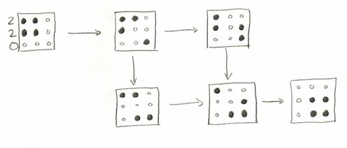
Given a partition (possibly with some zero parts), draw its Young diagram but replace the boxes with black dots and the “positions without boxes” with white dots. Don’t have any extra rows, but extra columns are okay. For instance, the partition $(2,2,0)$ corresponds to this picture

We then make moves according to the following rule, anytime we see a black dot in a TL corner of a square that’s otherwise white, we can move it to the BR corner:

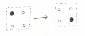
We make this move wherever possible until there are no more available. The set of all diagrams that can be obtained this way, starting with the partition $\lambda$ will be called, uncreatively, $\text{Black}(\lambda)$. To keep with our example, here is $\text{Black}((2,2,0))$:

Now it is time for some algebra: we are going to describe a polynomial in two sets of variables $X=x_1,\dots, x_r$, where $r$ is the number of rows; and $Y=y_1, y_2, y_3,\dots$ representing the columns. First, we define the weight of a diagram $\text{wt}(D)$ to be the product of every $x_i-y_j$, for all $i$ and $j$ such that there is a black dot in row $i$ and column $j$.

Finally, define the factorial Schur function $s_\lambda(X,Y)$ to be the sum of $\text{wt}(D)$ over all diagrams $D\in\text{Black}(\lambda)$. As a formula:

$$ s_\lambda(X,Y) = \sum_{D\in\text{Black}(\lambda)} ~~ \prod_{(i,j)\text{ is black}} x_i-y_j. $$

------

Littlewood-Richardson Polynomials

The reason that factorial Schur functions are called that is because if you plug $y_i=0$ for every $y$, the resulting polynomial is really, honestly, the Schur polynomial. Schur functions form a basis for the symmetric algebra, and so we might hope that the symmetric Schur functions are the basis for something. This hope turns out to be validated: it is a $\Bbb Z[Y]$-module basis of $\Lambda_n\otimes \Bbb Z[Y]$ (The last symbol there is polynomial algebra in the $y$-variables, and the symbol in the middle is a tensor product)

Because of that, this means that $s_\lambda(X,Y)s_\mu(X,Y)$ must be some linear combination, and so we can ask for the structure coefficients $C_{\lambda,\mu}^\nu(Y)$. We write the $Y$ there because in general these things can be an element in $\Bbb Z[Y]$; in other words, can be a polynomial in the $y$-variables. 

Since they specialize to the Littlewood-Richardson coefficients when $y_i=0$, we call these $C_{\lambda,\mu}^\nu$ the Littlewood-Richardson Polynomials

[ Because of the geometric interpretation of ordinary Littlewood-Richardson coefficients, we know that they are nonnegative integers; you may ask whether the LR-polynomials are also positive (in that all the coefficients are negative). The answer is no, but they are positive as polynomials in $z_i:=y_{i+1}-y_i$. ]

------

Polynomial Time

In 2005, one day after the other, two papers were posted to the arXiv, both claiming to have proven the following theorem:

Theorem (DeLoera–McAllister 2006, Mulmuley–Narayanan–Sohoni 2012*). There is an algorithm for determining whether or not the Littlewood-Richardson coefficient $c_{\lambda,\mu}^\nu=0$ in polynomial time.

If you’re not super familiar with “polynomial time”, feel free to substitute the word “quickly” anywhere you see it; this isn’t necessarily true but it’s a respectable approximation.

This naturally raises the question of whether the Littlewood-Richardson polynomials can also be determined to be zero or not in polynomial time. As the title of the talk suggests— and as Adve, Robichaux, and Yong proved— the answer is yes. The rest of this section is devoted to a proof sketch.

There is a celebrated proof due to Knutson–Tao which proves the so-called saturation conjecture, that $c_{\lambda,\mu}^\nu=0$ if and only if $c_{N\lambda,N\mu}^{N\nu}=0$ for all $N$. At this point, Yong talked a little bit about the history of that conjecture: 

In the 19th century, people were asking this question about Hermetian matrices.

In 1962 Horn conjectured a bunch of inequalities which resolved the question. 

In 1994 Klyachko solved the problem, but didn’t use Horn’s inequalities.

Soon after, it was realized that the saturation conjecture was sufficient to prove Horn’s inequalities.

In 1998, Knutson and Tao published their proof.

The argument they made in this paper was refined by a 2013 theorem of a different ARY team: Anderson, Richmond, and Yong. They showed that the analogous statement is true for the Littlewood–Richardson polynomials: $C_{\lambda,\mu}^\nu(Y)=0$ if and only if $C_{N\lambda,N\mu}^{N\nu}(Y)=0$ for all $N$. 

The major innovation made by the new ARY team (Adve, Robichaux, and Yong) constructed a family of polytopes $P_{\lambda,\mu}^\nu$ with the following properties: 

scaling the polytope by a factor of $N$ is the same as scaling the partitions by a factor of N, i.e. $P_{N\lambda,N\mu}^{N\nu} = NP_{\lambda,\mu}^\nu$,

and the crucial bit: $P_{\lambda,\mu}^\nu$ has an integer lattice point if and only if $C_{\lambda,\mu}^{\nu}(Y)\neq 0$

In particular, this implies that the “polynomial saturation conjecture” can be used to reduce the question of $C_{\lambda,\mu}^{\nu}(Y)\neq 0$ to figuring out whether $P_{\lambda,\mu}^\nu$ is the empty polytope. And this, finally, is a problem which is known to be solvable in polynomial time, which concludes the proof.

------

[ * The dates listed above are the publication dates of the papers that the two teams wrote. “So that tells you something about publishing in mathematics”, Yong says. Perhaps, but... I’m not sure what. I’m assuming that what he was getting at is this: The names in the latter team are nothing to scoff at, by a long shot; I mean, I have heard all five of these names before in other contexts. But the prestige associated to the names in the former team might have made that paper subject to less scrutiny than the latter. Or perhaps he just meant that the capricious turns of fate can turn what “should be” a short procedure into a long one. ]

[thousandmaths]

If you ever come back to the world of tumblr, @ryanandmath, I’d like to hear what your thoughts are, since I’d guess you’ve taken a qualifying exam or two by now :) 

In absence of that, I’ll say that I had similar thoughts to you when I started grad school, including when I was studying for the real analysis exam. But nowadays I do mostly agree with OP: my written quals were pretty darn “memorize-able”.

In particular, I offer this anecdotal evidence: I think the exam where I went in with the worst preparation was algebra (either for the subject matter or for the exam), and that was also the only one where I felt that I might have been able to finish if I’d had another hour.

On the other hand, I was way more prepared for topology, from the taking-an-exam point of view, than I was for real analysis. But I had a lot more background in real analysis than I had in topology, and consequentially I found the test easier.** I guess I just bring this up to say that— despite the similarities— I found the written quals not as easily gameable, nor as amenable to “do problems until your eyes bleed” quasi-cramming, as was the GRE subject test.

------

I don’t want to generalize too quickly: I know that UMN was in the process of trying to make its written quals a little more predictable— except that now there is one guy responsible for writing three of the four exams and it’s clear that he doesn’t buy into this idea as the people he took over from.

For the differential side of topology, which I have never really learned to my satisfaction (despite my attempts*), this predictable structure really paid off for me: in particular, I was pretty darn sure there would be a question about computing Lie brackets, and there would be one asking me whether a given form was exact, and so on.

I also know that UMN doesn’t use the written quals as a weed-out mechanism, which is not universally true. If anything can be said to be that, it would be the oral quals instead, but that is a completely different style of exam.

------

* Actually, the phenomenon I’m describing can maybe be seen clearly just by going through my writeups in that tag. You can see pretty clearly when a new guy started writing, but within the two “blocks”, everything is pretty consistent.

** My studying for the real analysis exam (which, however, I had considerable background in) was less about solving problems and more about just looking over the old exams and seeing what the “usual tricks” were.

For instance, most Prove/Disprove real analysis questions

about functions, could be reliably tested against Cantor’s staircase

about sets with weird measure properties, could be reliably tested against the fat Cantor set or a set containing every rational with nonzero-measure complement

about Hilbert spaces, would reliably benefit from using 

Most inequalities needed to use Hölder, most "evaluate this series” questions were really about Parseval’s theorem, and there was always a question testing the hypotheses of Fubini’s theorem.

But last spring the new guy was writing real analysis and so... yeah that strategy wouldn’t have worked very well at all. So: a vague idea of departmental politics + who wrote which exams and when; these are not bad ideas for contextualizing what you’re studying.

Qualifying exams in mathematics

After reviewing past tests from both my university and others, I’ve determined that written qualifying exams in mathematics graduate programs are like the math subject GRE on crack.

For the math subject GRE (note: not the math portion of the general GRE), the best way to prepare is:

1) Read the Princeton review book to remember how to do calculus, differential equations, and linear algebra. 

2) Do problems until your eyes bleed, then do some more (including taking all of the available practice tests). 

This worked very well for me. There’s no time to think on the test if you want to answer all the questions – everything needs to be automatic, you need to be able to solve every problem on sight. 

My approach to my upcoming qualifying exam has been basically the same, expect step 1 is has been replaced by “review everything on the syllabus.” Most of which I purportedly know, but have forgotten. I have yet to start step 2, but hope to get there soon. 

Some thoughts:

Many of the problems that appear on these exams are (like the GRE, like the SAT, etc) variations on well-known themes. For example, if your exam covers complex analysis, there will always be an integral you need to do by residues. Always. And if your exam covers algebra, you will almost always need to compute a Galois group. There are less obvious examples, too. I’ve seen the example from Dummit and Foote about counting monic irreducible polynomials of a fixed degree a few times, for instance. 

The best way to identify these is probably to mass-solve past exams and note the patterns. But generally, I’m making it my goal to know every to do everything on these lists (see here for the complex analysis list, for example). 

Knowing about messy proofs of hard theorems seems basically pointless. For example, no qualifying exam asks about proving the fundamental theorem of Galois theory, or the homotopy version of Cauchy’s theorem, etc. You DO need to know how to prove the simple stuff, but these are classic and you can see them coming a mile away – a finite multiplicative subgroup of a field is cyclic, Liouville’s theorem, the fundamental theorem of algebra, etc. 

Once you solve enough problems, a lot of the test questions you can see how to solve immediately (e.g. “Oh, right, this integral needs to be done by residues”) which allows you to save time for the trickier ones. Like the math GRE, you definitely do NOT want to spend time thinking about every question. You’ll run out of time, get stuck, etc. 

[thousandmaths]

Defining Equations of Rees Algebras

This talk was given by Claudia Polini at the 2017 CA+ conference. This post will not attempt to be elementary.

------

Rees Rings

The scope of the talk was ostensibly rather modest: “There is very little that we can say in general [about Rees rings]. This talk is about what can be said in some general situations.”

The sorts of “things” that we were trying to talk about was to determine when a certain ideal is of “fibre type”; to explain what this means and why we care about it requires rather more setup.

Let $k$ be a field and $R=k[x_1,\dots, x_d]$ be a polynomial ring. Given a bunch of homogeneous polynomials $f_1,\dots, f_n$ of degree $\delta$, consider the map $f=[f_1 : \dots : f_n]$ sending $k\Bbb P^{n-1}$ to $k\Bbb P^{n-1}$. Let the coordinate ring of the image— i.e. the collection of all polynomial functions on the image— be denoted $A(X)$. This ring fits into a short exact sequence

$$ 0 \to I(X) \to k[y] \to A(X) \to 0 $$

for some $k$-algebra $I(X)$. 

The story so far is very biased in favor of the image. But we may gain more information by looking at, instead of $A(X)$, the following analogous setup: let $I=(f_1,\dots, f_n)$ be the ideal that these X generate, and define the Rees ring $\mathcal R(I)$ to be $R[It]$. The Rees ring also fits into a short exact sequence

$$ 0 \to J \to k[x,y] \to \mathcal R(I) \to 0. $$

One can naturally identity $I(X)\subset J$, and the question is: if you know $I(X)$, can you determine $J$. And the answer is no, but you can if the ideal $I$ has fibre type.

------

Ideals of Fibre Type

The Rees ring also fits into a different short exact sequence, as a quotient of the symmetric algebra in the $f$s:

$$ 0 \to \mathcal A \to S(I) \to \mathcal R(I) \to 0. $$

This turns out to be very useful, because it gives several equivalent descriptions of what it means to be of fibre type: in particular, $\mathcal A= I(X)\cdot S(I)$, or also that $J$ is generated in degrees $(*,1)$ and $(0,*)$. This notation means that the $x$-degree can be whatever, but if it is not zero then the $y$-degree is forced to be $1$.

At this point, Polini did some technical work on the board that I didn’t follow, but her conclusion was that we were going to assume that $\mathcal A$ is a local cohomology module, namely $\mathcal A = H_{\mathfrak m}^0(\Lambda(I(\delta)))$

[ I believe that the $(\delta)$ notation means to construct an ideal which is the same as a set, but has a different notion of “degree”: all degrees are supposed to be shifted downward by $\delta$. Or perhaps upward... I was never clear what the goal of the degree shifting was supposed to be in this talk. ]

In this case, we have an even more workable characterization of fibre type: $\mathcal A_{\bullet, j}$ is generated in degree $0$ for all $j$.

------

Approximate Resolutions

It turns out that, under the local cohomology assumption we made before, the problem is completely solved if we had a minimal free resolution of the symmetric powers $\text{Sym}_j(I(\delta))$. [ No, I don’t know why. ]

Unfortunately, this will never happen because computing minimal free resolutions of symmetric powers is too hard. So instead we may hope for an approximate resolution. This is where, instead of a complex of free modules, we ask only that the complex contains finitely generated modules; and moreover we make no restrictions whatsoever on the higher homology groups. It’s worth noting, though, that in practice the power of approximate resolutions comes when you can assume some control on the higher homology groups; for instance $H_i(F_\bullet)\leq i$.

In 1979, Weyman published a construction which gives an approximate resolution $(C_{j,\bullet})$ for the $j^\text{th}$ symmetric power of $I(\delta)$, assuming you have a free resolution $(F_\bullet)$ of $I$. The details are not nearly as gory as you might expect:

$$ C_{j,t} = \bigoplus_{\alpha} D_{a_0}F_0 \otimes \Lambda^{a_1} F_1 \otimes D_{a_2}F_2 \otimes \cdots,$$

where the direct sum is taken over all compositions $\alpha=(a_1,\dots, a_k)$ with $\sum a_i = j$ and $\sum ia_i=t$.

In any case, this was the technique which Polini used to prove her result. That states, among other things, that $\mathcal A$ is generated in degrees at most $(d-1)(\text{reg}(I)-\delta)$ under some technical (and not insubstantial) restrictions on the ideal. The details of the conditions are important for the novelty of the work, but ultimately it is this control on the degrees which generated $\mathcal A$ that are the important theoretical advance.

At the end of her talk, she mentioned several other techniques which people are using to try to get bounds on these degrees. These will hopefully allow us to work with other, and perhaps larger, classes of rings.

[thousandmaths]

Distributing Points on the Sphere II

This is the second of two posts based on a talk given at Dmitriy Bilyk at our probability seminar (the first one is here). I don’t usually go to probability seminar, but have enjoyed Dmitriy’s talks in the past, and I didn’t regret it this time either :)

------

Semirandom Methods

In the previous post we defined the Riesz energy and the discrepancy, and we said that (deterministic!) sets which minimize either of these things should be said to be “uniformly distributed”. We also mentioned that in general, we don’t know very many deterministic methods for creating uniformly distributed points on the sphere.

Using these two measures, the situation does not improve much for purely deterministic methods. But it turns out that there are two semirandom methods that do pretty well by both measures. The easiest to describe, and the most successful, is called jittered sampling: take one point uniformly at random from each part of any “regular equal-area partition”, which is some technical thing that’s not important. What’s important are the results:

It on average achieves the upper bound in Beck’s theorem of $\approx N^{-\frac12-\frac1{2d}}\sqrt{\log N}$.

It doesn’t optimize the Riesz energies, but it “almost” does so, in a way that Bilyk did not describe.

Somewhat more complicated is the determinental point process. It seems that nowadays these are of pretty big interest to machine learning, idk. But I do know (or rather, Bilyk knows and so I can inform you) that it enjoys similar properties to jittered sampling, although it is not quite as good in the discrepancy sense (I believe it’s $\log N$ instead of $\sqrt{\log N}$, but don’t quote me).

He also talked about some work that he did with Feng Dai and my colleague and friend Ryan Matzke related to the Stolarsky Invariance Principle. I think this produces a third semirandom method which has similarly nice properties, although to be honest I did not really follow that part of the talk >.>

However, there has recently been a new theoretical advance which has allowed for the possibility of more deterministic methods; we’ll spend the rest of the post talking abut that.

------

Uniform Tessellations

Given two points $x$ and $y$ on the sphere, and a random hyperplane, the probability that the hyperplane separates them is the spherical distance between them $d(x,y)$ [technicality: on a sphere of appropriate radius such that the distance from the north to the south pole is $1$]. Motivated by this fact, we define a Hamming distance, relative to a given set $Z=\{z_1,\dots, z_N\}$, between two points $x$ and $y$ as

$$ d_Z(x,y) = \frac{\#\{z_i\in Z: z_i^\perp \text{ separates }x\text{ from } y\}}{N}.$$

[ Those of you who know a different notion of Hamming distance may be interested in reading Section 1.1 of this paper, which lays out the relationship very clearly. ]

For any fixed $x$ and $y$, as $N\to\infty$, the expected Hamming distance (over all sets of size $N$) converges to $d(x,y)$; this says that the Hamming distance is a fairly reasonable object. But what we actually want to do is the following: for any set $X\subset S^d$ (which need not be finite), we say that $Z$ induces a $\delta$-uniform tessellation of $X$ in the event that $\sup_X |d_Z(x,y)-d(x,y)| \leq \delta$.

The goal is to find small $N$ which admit sets that induce $\delta$-uniform tessellations of $X$; ideally the smallest such $N$. Of course finding large $N$ is not very hard: as the number of hyperplanes grows, there will eventually be some set which does this. Indeed, the existence of $\delta$-uniform tessellations can be understood as “speed of convergence” results for the convergence $d_Z\to d$ mentioned above.

Of course the answer is going to have to depend somehow on the geometry of $X$, and so our answer is going to have to depend on some quantified statement of how “bad” the geometry is. I do not wish to explain exactly how this is done, but Bilyk and Lacey were able to come up with two answers: 

Theorem (Bilyk–Lacey). There exist constants $C$ and $C’$ such that it is sufficient for either $N\geq C\delta^{-3}\omega(X)$, or $N\geq C’\delta^{-2}H(X)$.

Here, $\omega(X)$ is a classically studied geometric statistic, and $H(X)$ is a variant which Bilyk and Lacey invented.

This dramatically improves on previous results, and in particular gets us tantalizingly close to the (previously) conjectured optimal lower bound, which is $C\delta^{-2}\omega(X)$. You can see that this conjecture is sort of the combination of their two results: it takes the $-2$ power from the second bound but still uses the $\omega$ statistic. Unfortunately, Bilyk did not seem optimistic that there were many technical improvements that could be made to their idea. So breaking the $-3$ barrier with the $\omega$ is probably still in want of another innovation.

[thousandmaths]

I... guess I really shouldn’t be surprised that you’d written a post like this at one point, but (a) it’s neat! and (b) I’ve never actually read your blog on your blog because otherwise I would have known that you have a very neatly organized collection of your major sideblogs.

What IS the canonical momentum?

This post is going to try and explain the concepts of Lagrangian mechanics, with minimal derivations and mathematical notation. By the end of it, hopefully you will know what my URL is all about.

Some mechanicses which happened in the past

In 1687, Isaac Newton became the famousest scientist jerk in Europe by writing a book called Philosophiæ Naturalis Principia Mathematica. The book gave a framework of describing motion of objects that worked just as well for stuff in space as objects on the ground. Physicists spent the next couple of hundred years figuring out all the different things it could be applied to.

(Newton’s mechanics eventually got downgraded to ‘merely a very good approximation’ when quantum mechanics and relativity came along to complicate things in the 1900s.)

In 1788, Joseph-Louise Lagrange found a different way to put Newton’s mechanics together, using some mathematical machinery called Calculus of Variations. This turned out to be a very useful way to look at mechanics, almost always much easier to operate, and also, like, the basis for all theoretical physics today.

We call this Lagrangian mechanics.

What’s the point of a mechanics?

The way we think of it these days is, whatever we’re trying to describe is a physical system. For example, this cool double pendulum.

The physical system has a state - “the pieces of the system are arranged this way”. We can describe the state with a list of numbers. The double pendulum might use the angles of the two pendulums. The name for these numbers, in Lagrangian mechanics, is generalised coordinates.

(Why are they “generalised”? When Newton did his mechanics to begin with, everything was thought of as ‘particles’ with a position in 3D space. The coordinates are each particle’s \(x\), \(y\) and \(z\) position. Lagrangian mechanics, on the other hand is cool with any list of numbers can be used to distinguish the different states of the system, so its coordinates are “generalised”.)

Now, we want to know what the system does as time advances. This amounts to knowing the state of the system for every single point in time.

There are lots of possibilities for what a system might do. The double pendulum might swing up and hold itself horizontal forever, for example, or spin wildly. We call each one a path.

Because the generalised coordinates tell apart all the different states of the system, a path amounts to a value of each generalised coordinate at every point in time.

OK. The point of mechanics is to find out which of the many imaginable paths the system/each coordinate actually takes.

The  Action

To achieve this, Lagrangian mechanics says the system has a mathematical object associated with it called the action. It’s almost always written as \(S\).

OK, so here’s what you do with the action: you take one of the paths that the system might take, and feed it in; the action then spits out a number. (It’s an object called a functional, to mathematicans: a function from functions to numbers).

So every path the system takes gets a number associated with it by the action.

The actual numbers associated with each path are not actually that useful. Rather, we want to compare ‘nearby’ paths.

We’re looking for a path with a special property: if you add any tiny little extra wiggle to the path, and feed the new path through the action, you get the same number out. We say that the path with this special property is the one the system actually takes.

This is called the principle of stationary action. (It’s sometimes called the “principle of least action”, but since the path we’re interested in is not necessarily the path for which the action is lowest, you shouldn’t call it that.)

But why does it do that

The answer is sort of, because we pick out an action which produces a stationary path corresponding to our system. Which might sound rather circular and pointless.

If you study quantum field theory, you find out the principle of stationary action falls out rather neatly from a calculation called the Path Integral. So you could say that’s “why”, but then you have the question of “why quantum field theory”.

A clearer question is why is it useful to invent an object called the action that does this thing. A couple of reasons:

the general properties actions frequently make it possible to work out the action of a system just by looking at it, and it’s easier to calculate things this way than the Newtonian way.

the action gives us a mathematical object that can be thought of as a ‘complete description of the behaviour of the system’, and conclusions you draw about this object - to do with things like symmetries and conserved quantities, say - are applicable to the system as well.

The Lagrangian

So, OK, let’s crack the action open and look at how it’s made up.

So “inside the action” there’s another object called the Lagrangian, usually written \(L\). (As far as I know it got called that by Hamilton, who was a big fan of Lagrange.) The Lagrangian takes a state of the system and a measure of how quickly its changing, and gives you back a number.

The action crawls along the path of the system, applying the Lagrangian at every point in time, and adding up all the numbers.

Mathematically, the action is the integral of the Lagrangian with respect to time. We write that like $$S[q]=\int_{q(t)} L(q,\dot{q},t)\dif t$$

What can you do with a Lagrangian?

Lots and lots of things.

The main thing is that you use the Lagrangian to figure out what the stationary path is.

Using a field of maths called calculus of variations, you can show that the path that stationaryises the action can be found from the Lagrangian by solving a set of differential equations called the Euler-Langrange equations. If you’re curious, they look like $$\frac{\dif}{\dif t}\left(\frac{\partial L}{\partial \dot{q}_i}\right) = \frac{\partial L}{\partial q_i}$$but we won’t go into the details of how they’re derived in this post.

The Euler-Lagrange equations give you the equations of motion of the system. (Newtonian mechanics would also give you the same equations of motion, eventually. From that point on - solving the equations of motion - everything is the same in all your mechanicses).

The Lagrangian has some useful properties. Constraints can be handled easily using the method of Lagrange multipliers, and you can add Lagrangians for components together to get the Lagrangian of a system with multiple parts.

These properties (and probably some others that I’m forgetting) tell us what a Lagrangian made of multiple Newtonian particles looks like, if we know the Lagrangian for a single particle.

Particles and Potentials (the new RPG!)

In the old, Newtonian mechanics, the world is made up of particles, which have a position in space, a number called a mass, and not much else. To determine the particles’ motion, we apply things called forces, which we add up and divide by the mass to give the acceleration of the particle.

Forces have a direction (they’re objects called vectors), and can depend on any number of things, but very commonly they depend on the particle’s position in space. You can have a field which associates a force (number and direction) with every single point in space.

Sometimes, forces have a special property of being conservative. A conservative force has the special property that

depends on where the particle is, but not how fast its going

if you move the particle in a loop, and add up the force times the distance moved at every point around the loop, you get zero

This is great, because now your force can be found from a potential. Instead of associating a vector with every point, the potential is a scalar field which just has a number (no direction) at each point.

This is great for lots of reasons (you can’t get very far in orbital mechanics or electromagnetism without potentials) but for our purposes, it’s handy because we might be able to use it in the Lagrangian.

How Lagrangians are made

So, suppose our particle can travel along a line. The state of the system can be described with only one generalised coordinate - let’s call it \(q(t)\). It’s being acted on by a conservative force, with a potential defined along the line which gives the force on the particle.

With this super simple system, the Lagrangian splits into two parts. One of them is $$T=\frac{1}{2}m\dot{q}^2$$which is a quantity which Newtonian mechanics calls the kinetic energy (but we’ll get to energy in a bit!), and the other is just the potential \(V(q)\). With these, the Lagrangian looks like $$L=T-V$$and the equations of motion you get are $$m\ddot{q}=-\frac{\dif V}{\dif q}$$exactly the same as Newtonian mechanics.

As it turns out, you can use that idea really generally. When things get relativistic (such as in electromagnetism), it gets squirlier, but if you’re just dealing with rigid bodies acting under gravity and similar situations? \(L=T-V\) is all you need.

This is useful because it’s usually a lot easier to work out the kinetic and potential energy of the objects in a situation, then do some differentiation, than to work out the forces on each one. Plus, constraints.

The Canonical Momentum

The canonical momentum in of itself isn’t all that interesting, actually! Though you use it to make Hamiltonian mechanics, and it hints towards Noether’s theorem, so let’s talk about it.

So the Lagrangian depends on the state of the system, and how quickly its changing. To be more specific, for each generalised coordinate \(q_i\), you have a ‘generalised velocity’ \(\dot{q}_i\) measuring how quickly it is changing in time at this instant. So for example at one particular instant in the double pendulum, one of the angles might be 30 degrees, and the corresponding velocity might be 10 radians per second.

The canonical momenta \(p_i\) can be thought of as a measure of how responsive the Lagrangian is to changes in the generalised velocity. Mathematically, it’s the partial differential (keeping time and all the other generalised coordinates and momenta stationary): $$p_i=\frac{\partial L}{\partial \dot{q}_i}$$They’re called momenta by analogy with the quantities linear momentum and angular momentum in Newtonian mechanics. For the example of the particle travelling in a conservative force, the canonical momentum is exactly the same as the linear momentum: \(p=m\dot{q}\). And for a rotating body, the canonical momentum is the same as the angular momentum. For a system of particles, the canonical momentum is the sum of the linear momenta.

But be careful! In situations like motion in a magnetic field, the canonical momentum and the linear momentum are different. Which has apparently led to no end of confusion for Actual Physicists with a problem involving a lattice and an electron and somethingorother I can no long remember…

OK a little maths; let’s grab the Euler-Lagrange equations again: $$\frac{\dif}{\dif t} \left(\frac{\partial L}{\partial \dot{q}}\right) = \frac{\partial L}{\partial q_i}$$Hold on. That’s the canonical momentum on the left. So we can write this as $$\frac{\dif p_i}{\dif t} = \frac{\partial L}{\partial q_i}$$Which has an interesting implication: suppose \(L\) does not depend on a coordinate directly, but only its velocity. In that case, the equation becomes $$\frac{\dif p_i}{\dif t}=0$$so the canonical momentum corresponding to this coordinate does not change ever, no matter what.

Which is known in Newtonian mechanics as conservation of momentum. So Lagrangian mechanics shows that momentum being conserved is equivalent to the Lagrangian not depending on the absolute positions of the particles…

That’s a special case of a very very important theorem invented by Emmy Noether.

The canonical momenta (or in general, the canonical coordinates) are central to a closely related form of mechanics called Hamiltonian mechanics. Hamiltonian mechanics is interesting because it treats the ‘position’ coordinates and ‘momentum’ coordinates almost exactly the same, and because it has features like the ‘Poisson bracket’ which work almost exactly like quantum mechanics. But that can wait for another post.

Coming up next: Noether’s theorem

Lagrangian mechanics may be a useful calculation tool, but the reason it’s important is mainly down to something that Emmy Noether figured out in 1915. This is what I’m talking about when I refer to Lagrangian mechanics forming the basis for all the modern theoretical physics.

[OK, I am a total Noether fangirl. I think I have that it common with most vaguely theoretical physicists (the fan part, not the girl one, sadly). To mathematicians, she’s known for her work in abstract algebra on things like “rings”, but to physicists, it’s all about Noether’s Theorem.]

Noether’s theorem shows that there is a very fundamental relationship between conserved quantities and symmetries of a physical system. I’ll explain what that means in lots more detail in the next post I do, but for the time being, you can read this summary by quasi-normalcy.

[thousandmaths]

Distributing Points on the Sphere I

This is the first of two posts based on a talk given at Dmitriy Bilyk at our probability seminar. I don’t usually go to probability seminar, but have enjoyed Dmitriy’s talks in the past, and I didn’t regret it this time either :)

------

Unsatisfactory Methods

Here is how not to pick a point uniformly on the sphere: don’t pick its polar and azimuthal angles uniformly. This doesn’t work because it will incorrectly bias things toward the poles. 

What does work is to pick the polar angle and $z$-coordinate uniformly.

So that was a short talk :P

The problem is that this cylindrical trick only works on the 2-sphere. There is no natural notion of “cylindrical coordinates” for higher-dimensional spheres, because how many coordinates do you take linearly and how many do you take as angles? 

Bilyk did not say this, but presumably no choice you can make, or at least no consistent choices that you can make for all $n$, such that you get a uniform distribution— otherwise it really would have been a short talk :P

What Bilyk did say is that there are several ways to choose points uniformly from a sphere, but “there are very few deterministic methods”. But before we can tackle these methods, we actually need to answer a more fundamental question: what does it mean to choose deterministically choose points uniformly? Generally “choosing uniformly” means sampling from a constant random variable, but that X is clearly not available to us here.

------

Riesz Energy

One way to go might be to minimize the Riesz energy. Whenever we have a collection of points $Z=\{z_1,\cdots z_N\}$, can write

$$ E_s = \frac{1}{N^2} \sum_i \sum_{j\neq i} \frac{1}{z_i-z_j}. $$

We see that if the $z_k$ are very close to each other, this energy is going to be large; a set $Z$ that makes the energy small will be one whose points are generally “as far from each other as possible”. Since it’s a sphere, you can’t get too far away, and so there’s an interesting optimization to be done here.

So this seems nice, but there’s a problem. It turns out that minimizing the Riesz energy is just, like, stupendously hard. The best exact result we have was given in 2010, when Schwartz proved that $E_1$ is minimized for $N=5$ (!) by the triangular bipyramid.

(source)

To give some indication about why the problem is hard: the triangular bipyramid is not the minimizer for the Riesz energy with $N=5$ for all $s$. It is suspected that it minimizes it for all sufficiently small $s$; but one thing we know for sure that when $s$ gets large enough, the square pyramid is better.

Conjecture. There exists a critical value $s’$ such that for all $1\leq s<s’$, the triangular bipyramid minimizes $E_s$, and for all $s’<s$, the square pyramid minimizes $E_s$.

This conjecture is wide open: we don’t even know that the square pyramid minimizes $E_s$ for any value of $s$!

------

Discrepancy and a Theorem of Beck

Another, rather different way to measure the uniform-ness of a set $Z$ is by computing its discrepancy. The formal definition of discrepancy is really a lot scarier than necessary, so I won’t write it here. The idea is that if you pick any (measurable) set $S$, you can either

calculate the measure of the $S$, or

count how many of the points $z_i$ live inside $S$

Most of the time, these two numbers are going to be different, and the discrepancy $D(Z,S)$ is the difference between the numbers, divided by the number of points in $Z$. But this is not the most useful number because we have this extra data $S$ hanging around; the better idea is to let the discrepancy be the maximum of $D(Z,S)$ over all $S$ (technically the supremum).

Intuitively speaking, that if you were to have a $Z$ for which the discrepancy in the latter sense were small, then $Z$ looks “uniformly distributed”, even if $Z$ is deterministic.

However, measurable sets can look pretty wacky, and so in order to let geometry reign over set theory, it often helps to be a little more refined. Given a collection of sets $\mathcal S$, we say that the discrepancy $D(Z,\mathcal S)$ is the supremum of $D(Z,S)$ over all $S\in\mathcal S$. So it’s basically the same thing as what we did above, except that instead of doing all measurable sets, we only do the ones in the collection.

Figuring out optimal discrepancies is also not very easy, but people have over the years figured out strategies for determining asymptotic bounds. And even that tends to be pretty tough. For instance, if we’re considering things on the sphere, it may seem reasonable to look at $\mathcal S$ the collection of spherical caps:

(source)

What is the best available discrepancy in this setting? The answer, morally speaking, is that it’s “close to $1/\sqrt{N}$”, but it has a small dimensional correction:

Theorem (Beck 1984). For any positive integer $N$, there exist positive constants $C_0$ and $C_1$ such that

$$ C_0 N^{-\frac12-\frac1{2d}} \leq \inf_{|Z|=N} D(Z,\mathcal S) \leq C_1 N^{-\frac12-\frac1{2d}} \sqrt{\log N}, $$

where $\mathcal S$ is the set of spherical caps.

So you can always find a set $Z$ that does a little better, asymptotically, than $1/\sqrt{N}$; what exactly “a little” means depends on how high-dimensional your sphere is.

------

In the next post, we talk about more recent developments, including a third notion of uniform distribution which will bring us all the way to Bilyk’s work in the present day.

[thousandmaths]

This has been sitting in my drafts box for most of the summer, with the following comment:

sooooo can you answer the question? 

I didn’t actually write “the question” down because to me, the question posed by this gif is blisteringly obvious: Given an arbitrary graph, how many Eulerian trails does it have? (An Eulerian trail is what you think it is based on this picture: start at a vertex and draw all the edges in the graph without lifting your pen or crossing over an edge twice.)

At various points through the summer I’ve played around with this question, trying not-too-seriously to see if I couldn’t take it down. I didn’t expect it to be particularly difficult, since it is the counting problem whose decision problem is extremely easy. Namely, you can determine if a graph has any Eulerian trails by simply looking at the degrees of its vertices— the number of edges attached to each vertex. If all these numbers are even, or if exactly two of them are odd, then the graph doesn’t have an Eulerian trail. If not, there isn’t*. That’s just about as straightforward as it gets.

But now that the blog is getting pretty close to completion, I thought I’d try to resolve the question for real, so I started Googling around. I was surprised to discover this MSE question, where Gerry Meyerson pointed out that the Wikipedia page has a reference to a paper of Brightwell and Winkler. This paper proves that this problem is #P-complete— which is a technical word that means “really friggin hard”.

The proof is actually very short, when you get right down to it, clocking in at barely over a page. It is almost entirely elementary, too, except that in the very last line it uses the following “wait, why?” fact from number theory:

Fact (Hardy–Wright). For any $n \geq 4$, the product of the set of primes strictly between $n$ and $n^2$ is at least $n!2^n$.

The answer to “wait, why?” is clear in context: the authors prove that a certain number can be computed mod any prime in polynomial time. They can then use the Chinese remainder theorem to compute the number exactly.** And the only way this could possibly go wrong is if you needed to use too many primes, but the number-theoretic fact guarantees that you only need to use $\mathcal O(n^2)$ of them, that is, polynomially many. Which in turn means the entire computation of this number can be done in polynomial time!

------

[ * If you’ve not super familiar with graph theory, it may not be totally obvious that there are graphs which don’t have Eulerian trails, but in fact there are tons. Actually, the first problem ever considered in graph theory was the famous “Seven Bridges of Königsburg” problem, which boils down to showing that the following graph has no Eulerian trails:

If you try to draw one, you’ll see what goes wrong pretty quickly. Formalizing this into a careful argument that no possible way of tracing the edges gives an Eulerian trail, is considerably trickier. Unless, of course, you know the punchline that you can just count degrees, in which case it is obvious: every vertex has odd degree! ]

[ ** the number is potentially very exponential in $n=|V|$, so you can’t just take a prime larger than the number. ]