thepixelary

[thepixelary]

The Ultimate Blender Cycles Performance Guide - Part 2 - Software

For the next few weeks, we will be posting a series of articles summarizing our experience with the Cycles rendering engine for Blender. This series is the result of years of working at The Pixelary, combined with hundreds of hours of benchmarking. We hope you’ll find this to be a useful resource for you to get the most out of your production with Blender.

In Part 1 we discussed hardware, but short of buying a stack of CPUs and GPUs, what can we do to improve the rendering performance of Blender’s Cycles engine given the same hardware? This is Part 2 of the series, and we'll be focused on the software.

Effect of OS + Blender versions

Let’s first test different OS and Blender combinations using test files from the official Blender Benchmark Beta 2, which contains 6 scenes of varying complexity to give us an accurate representation of performance across a wide range of projects. The test is conducted on a Ryzen 2700x with 2 1080 Ti and 32GB of DDR3200 RAM.

Let's start with the baseline, a Windows 10 machine with the latest 1903 update running Blender 2.79a. We then ran the exact same scene through Blender 2.8, and then repeated the process in Ubuntu 19.04.

It's clear from the graph that Blender has improved quite a bit since the 2.79 days. We are getting a noticeable improvement in performance just by using the latest version of Blender. The results is even more promising for Linux, we see a 10-15% improvement in performance over Windows on the same hardware and Blender version. That means, compared to our baseline, a Blender 2.8 running in Linux is nearly twice as fast as 2.79 running in Windows!

Can we do even better? You bet! There is a paid build of Blender called E-Cycles that uses various optimizations to deliver an even faster GPU render. The output of this build is not pixel-identical to the official build, but is visually indistinguishable and should be sufficient for most of the use cases. Note that CPU rendering speed is not affected in this build.

From the chart above, we can see that E-Cycles makes our Windows machine as fast as Linux.

This chart doesn’t tell the full story either, from our testing, E-Cycles actually offers even bigger performance improvement in simpler scenes, We’ve often seen 1.5x to 2x performance improvement in some scenes.

Micro Optimizations

What we discovered during our testing is that different scenes sees different amount of speedups, so it’s best to benchmark with the actual scene you are working on. There are also tons of micro optimizations one can do to Windows and Linux that can potentially speed up the rendering by a few percentage. In our opinion, these tweaks are not worth pursuing.

GPU Rendering Quirks

With GPU rendering, there are a few other issues to keep in mind. Apart from the memory limitation already mentioned, you will also likely experience stutter and lags on the desktop when the GPU is busy rendering (and thus not available for drawing the user interface). This can be alleviated by having multiple GPUs, and set one of which to be only used for display, not rendering.

Another quirk of running GPU rendering is that Windows doesn't like it when the GPU is kept busy for more than a few seconds, which makes Windows think the GPU has crashed. When this happens it will hard-reset the GPU, which will cause the render to actually crash. Luckily, we can get around this watchdog behaviour by increasing the timeout threshold to a larger value, like 30 or 60 seconds. This process is detailed in the Substance Painter documentation, which also uses the GPU for long computations.

The takeaway from this is that using optimized software and OS can often offer multiple times the performance increase. So make sure to keep your OS, driver, and software up to date!

[thepixelary]

The Ultimate Blender Cycles Performance Guide - Part 1 - Hardware

For the next few weeks, we will be posting a series of articles summarizing our experience with the Cycles rendering engine for Blender. This series is the result of years of working at The Pixelary, combined with hundreds of hours of actual benchmark. We hope you’ll find this to be a useful resource for you to get the most out of your production with Blender.

Being an open source software, Blender will always be improving. The results we presented here are tested on Blender 2.80 Beta and should be valid for Blender 2.79 as well. We’ll try our best to keep this up-to-date as new features are rolled out.

Improving rendering performance is always the hot topic of any CGI work. Faster rendering means more iterations, more creativity, happier artists, and happier clients. But what we learned is that getting the fastest rendering is not a trivial task and cannot be accomplished by tuning on a few settings at the end, it requires a deep understanding of how Cycles work, and making the right decision every step of the way, from picking the right hardware, the right software, to creating projects in a way that makes the most out of the limited resources you have.

Hardware and System

Many studio artist don't think about the underlying hardware they are using - it’s just a mean to an end. But having a good understanding of how hardware and software work together can help you learn how to optimize for both.

We are focused on rendering performance of Cycles, which is entirely dependent on the performance of the compute cores (CPU or GPU).

CPU vs GPU Rendering

Cycles can perform the rendering on the CPU as well as the GPU (or both at the same time!). When we look at the performance per dollar, you might be surprised to find that CPU and GPU are quite similar. A $1000 CPU renders at roughly the same speed as a $800 GPU, this is especially true for high-core-count CPUs such as AMD’s Ryzen and Threadripper line. The biggest drawback for GPU rendering is that your scene has to fit within the memory of your GPU, which tend to be quite small (8 to 16GB as of 2019).

Even though Blender 2.8 has support for out of core textures when rendering with GPU, meaning the entire scene doesn't have to fit within the size of the video memory, we still run into some stability issues with this setup. So GPU rendering is only recommended if the projects you work with are relatively small.

Takeaway: GPU offers slightly better performance per $ compared to CPU, but GPU rendering is limited by video memory.

Multi-GPU rendering

One benefit of GPU rendering is that it is much easier to get additional performance. You can easily put 4 GPUs into a computer and get 4x the speed up. They don’t even have to be the same GPU. Our studio buy a new GPU roughly every 12 months to add to the systems and rotate out the oldest one. This way we always get blistering performance without paying a huge upfront cost for staying on the bleeding edge.

To achieve this level of performance in a single box with CPU would require a significantly more expensive motherboards that accepts multiple CPUs. Not practical.

Keep in mind that when rendering with multiple GPUs, video memory size are not cumulative, instead you are limited to the smallest video memory available. So if you have a 8GB GPU and a 12GB GPU working together, you be limited to 8GB of usable video memory. Not 20GB.  (Side note, Nvidia Quadro cards with NVLink could potentially do memory pooling, but they are not tested with Blender as of 2019)

Takeaway: GPU is easier to scale up for more performance simply by adding more cards.

CPU vs CUDA vs OpenCL

In order to support multiple compute devices, Blender 2.8 has 3 rendering kernels: CPU, CUDA for Nvidia GPU, and OpenCL for AMD Radeon GPUs. As of mid 2019, all three pathway are largely at feature parity. Meaning there shouldn’t be much visible differences between the image produced by these 3 different class of devices.  Of course, as more features are added to Blender, it’s always possible that certain features are will be available on CPU first.

What about Geforce RTX or other hardware raytracing GPUs? Currently Cycles does not take advantage of the RT cores in the Nvidia RTX series, so you will not see any dramatic improvement in performance. But this could change in the future. When it does, it will make GPU rendering so much more attractive than CPU.

Takeway: CPU is the most feature-complete render kernel, but CUDA and OpenCL are practically identical for 99% of the use cases.

Tweaking and Monitoring

We like to keep an eye on our systems. The Windows Task Manager is actually pretty decent at this, with the most recent update you can even see your GPU utilization. With a simple tool like this, you can catch the system before it runs out of memory, or simply see whether a program is limited by the CPU, GPU, or storage speed.

If you are adventurous and would like to going further in optimizing your hardware, there are various software and bios settings that allows you to overclock your AMD CPU/GPU, Intel CPU, or Nvidia GPU. Normally adjusting these settings outside of their spec is not recommended, especially on a production machine. But instead of going for maximum performance via overclocking, we typically try to lower the power limit or voltage of these chips. By doing so, we lower the operating temperature of our CPU/GPU and actually end up boosting performance while reducing the noise and heat output of our computer.

Luckily, with software based overclocking, it’s pretty darn hard to actually damage your computer permanently. The worst that can happen is some data-loss due to unexpected crashes.

Takeaway: A well-tuned machine can run 10-20% faster than in stock configuration. But this tuning requires some knowledge of hardware and comes with certain risks.

Cloud Rendering

AWS, Azure, Google Cloud, all offer incredibly competitive price for computing tasks. There are also a huge number of premade render services available for hire. However, being a small studio, we haven’t had a lot of need for cloud rendering. We find that giving the artist the fastest workstation under their feet is far better for their productivity than offering burst performance via the cloud. For us, even animated shots can be typically rendered within 16 hours, which means the artists can fire it off when they are done for the day and it’s ready for review the next morning. Keeping the content local means less iterations due to bad render configurations or missing files.

Takeaway: Might be great for some studios or freelancers, but to each of their own.

Other Considerations

This article made no mention of memory, storage, or networking capabilities of a system. We work with the philosophy that these parts should just get out of the way for the computing to happen, so make sure there is enough of each to not cause a bottleneck.

Conclusion

If you want to work as efficiently as possible, start by understanding the hardware you are using.  Puget Systems has tons of benchmarks across a wide range of creative applications.  A 3 year old Quadro GPU or Xeon might not be as fast as you think compare to a modern consumer device, always look at benchmarks, and benchmark your own system.

Next week, we’ll dive into OS and custom builds of Blender.

[thepixelary]

Blender for Computer Vision Machine Learning

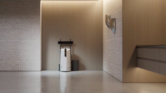
A while ago, we were approached by Greppy.co for a very unique application of our CGI skills. Greppy is a startup that specializes in autonomous robots for cleaning washrooms. While the robotic hardware is still in development, Greppy needed a way to train their computer vision software to quickly and accurately recognize toilet seats through machine learning (ML).

Object classification, more commonly known as object recognition, is simple: supply the computer with enough photos of something, along with a descriptor of exactly where it is in each photo, and the computer will learn how to recognize it. This process takes thousands or even tens of thousands of photos. So the main challenge is, how to you find enough images to feed the ML algorithm? While it might be possible to rely on a Google Image search, we still need to tag individual photos with the outline of the toilet seat. This tagging is a manual process that has to happen for each of the photos we need.

Rather than collecting real photos and tagging them manually, we decided it would be faster to generate all the images with CGI, and then feed those images back into the computer. This approach has a few distinct advantages over crowd-sourced photo labelling:

We can generate pixel-perfect masks and depth data for the ML system automatically.

We can cover a comprehensive range of washroom design, layout, lighting and colors.

The image generation system we build can be used for other things in the future.

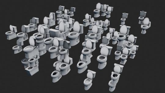
So with these goals in mind, we set out to create a 3D washroom in Blender. Our virtual robotics training scene consists of 40+ real toilet models and layouts. We even included sinks and tubs to make sure that the ML algorithm doesn’t overfit the data and think everything that’s shiny and can hold water is a toilet bowl.

With all the assets ready, we created a script that can iterate through all the combinations of these assets.  We also randomly position the camera so that we cover all the possible angles at which the robot can perceive the subject. Once you combine all the variations, the number of images it can produce is staggering. A full run would consists of 40 toilets x 3 bins x 3 walls x 3 floors x 8 lighting setups x 10 cameras, which is over 86,000 images!

Here is a small selection of the output:

Because the output image will be used for computer vision, we put extra emphasis on lighting accuracy to make sure the image resembles the real world as much as possible. The Cycles rendering engine was chosen to deliver photorealistic renderings at a relatively fast speed. Because we needed to render thousands of images, very aggressive optimizations were used to make sure only details that can be picked up by the 500x500 final render are included.

One of the biggest benefits of CGI training data is our ability to generate perfect masks and depth data out of the render, both of which are crucial for many machine learning applications which rely on depth data from stereo cameras to aid in the object recognition process.

While the goal of most CGI is to produce something that’s aesthetically pleasing, our goal here is speed over details.

A typical beauty render needs enough samples to get a clean image, but we were able to get away with using very few samples and heavy denoising to get a clean-enough image. This imperfect output actually make the computer vision system better at identifying objects under challenging lighting scenarios.

For the same reason, we intentionally turned off the new ‘Filmic’ LUT in Blender, and went back to the much less pleasant looking sRGB OETF transform. The reason behind that is the camera we are training for does not have the dynamic range nor light responsive of a high-end film camera. In fact, it behaves much more like a cellphone camera, with blown out highlights and all, so we intentionally lowered the color fidelity in order to mimic the response curve of the actual robotic camera.

When it comes to the final rendering, we used several GPU instances provided by Google Compute Platform. The images were rendered in only a few short days.

The end result is fantastic! Greppy was able to successfully integrate these images into their machine learning pipeline and is already seeing great results in producing a neural network that accurately and quickly identifies toilet seats of all shapes and sizes.

This image generation system that we setup can be adapted to train computer vision systems for other industries and uses. The speed at which we can produce a large number of relevant images is staggering, and at a much lower overall cost than crowdsourcing images.

[thepixelary]

Improving performance of Blender’s Cycles rendering on Windows 10

Here at the Pixelary, we try to squeeze every bit of performance out of our hardware. And one thing we noticed is that when using CUDA GPU rendering, Blender’s Cycles renders significantly faster on Linux than on Windows. What gives?

The above test is run on a  single Titan X (Maxwell) GPU with an AMD Ryzen 7 CPU. But it isn’t limited to Maxwell generation GPUs either. Here is the result for a 1080Ti (Pascal generation):

We get the same slow performance on Windows regardless of whether the GPU is used for display or not, nor does it matter if the we render from the command line.

Not willing to accept that Windows 10 is ‘simply slower’. We set out to find a solution.

Turns out, when doing GPU rendering on Windows 8 or above, any command that’s issued by Blender has to go through the WDDM, or Windows Display Driver Model. This driver layer is responsible for handling all the display devices, but it often adds a significant overhead to computing tasks. This model is a core component of Windows and cannot be disabled simply.

Luckily, the smart people at Nvidia already has a solution for it. To by pass the WDDM completely, we need to set the GPU as a “Tesla Compute Cluster”, or TCC for short. Once we enabled that, the GPU is no longer visible as a display device under Windows. But it’s still accessible by all CUDA apps. We than ran all the Blender benchmark again and here is the result:

With TCC enabled, Windows performance is exactly the same as Linux!

Now, here is the bad news. TCC is only available on Geforce Titan and Geforce Quadro line of GPUs, it is not available for Geforce GTX series. And it only works if you have another GPU to drive the display output (since TCC devices cannot be used to drive any display). But if you have to stick to a Windows environment and have a separate GPU, TCC might just be what you need to get that extra 30% performance back.

Rendering with AMD devices using OpenCL does not have this performance discrepancy.

So now we know WHY Windows is slower, we still would like to see ways to work around the WDDM limitation through more efficient kernels or reduced called to the WWDM. This will ensure that all Geforce users who cannot enabled TCC will still benefit from a speedy render.

[thepixelary]

This is our latest creation. Based on a CC0 model from Blendswap, we recreated the materials and shaders from scratch to arrive at this photorealistic render of a cheeseburger.

The project started as a test of ProRender for Blender. We knew food is extremely tricky to get right, and we wanted to really push the rendering engine. I think we are very happy with how this turned out.

[thepixelary]

Siggraph 2017 Recap

We just spent the last week in Los Angeles for the annual SIGGRAPH conference. Here is a quick summary of some of the notable things we saw:

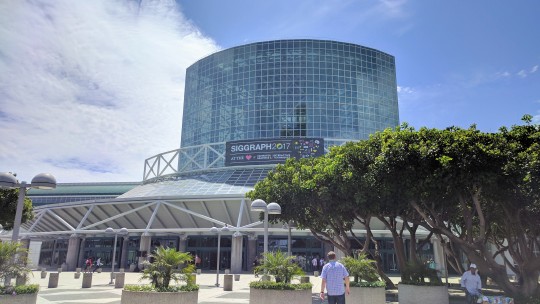
Blender is going strong! For 3 days, the Blender booth was always crowded despite its location. Tons of Blender users dropped by to say hi,  and even more people were genuinely surprised to learn what it can do.

This year is all about VR! Lots of headsets, cameras, and tracking technologies were on display. Price and ease of use will ultimately be the deciding factor for many of these.

3D printing is still being shown, and it’s much more refined than before, The focus is now on increased speed, wider material selection, and resolution.

AMD is back in the game baby! AMD showcased tons of their new hardware including Threadripper CPU and Vega GPU based workstations. They also generously provided all the hardware used by the Blender booth.

When it comes to computing performance, It’s all about density. A single tower can now easily pack 32 threads, 4 high end GPUs, and insane amount of ram.  A 2U rack can house 10 GPUs and cost as much as a new car.

The push toward realtime graphics continues. VFX studios are borrowing game-like features to add interactivity to their pipeline. All pathtracers can run in realtime at this point thanks to years of optimization and ever faster hardware.

Wide gamut and HDR displays were not as prevalent this year, maybe because the consumers haven’t really seen the benefit of these technologies, which is really something that you can only experience in person. Or maybe it’s because the content production pipeline for wide color is still a mystery to a lot of artists. Mastering images outside of the sRGB colorspace is hard to get right, and incredibly easy to get wrong.

Siggraph veteran Pixar and Unreal are the two notable companies that did not have a public exhibit area this year.

For the first time(and hopefully the last), we saw fidget spinners making an appearance as giveaways.

That’s about it, see you at next year’s SIGGRAPH in Vancouver!

[thepixelary]

We are very excited about Blender 2.8′s new Eevee viewport. This is rendered in the viewport in realtime.

[thepixelary]

Google Expeditions: VR for the Classroom

The concept of virtual-reality has been around for many decades now. However it is only in the last few years that technology has matured enough for VR to really take off.  HTC Vive and Oculus Rift are leading the way for high-end VR experiences, and mobile solutions such as Google Daydream and Samsung Gear VR provide simple and affordable solutions for the masses.

We had the amazing opportunity to contribute content to the Google Expeditions project. Google Expeditions is a VR learning experience designed for classrooms. With a simple smartphone and a Cardboard viewer, students can journey to far-away places and feel completely immersed in the environment. This level of immersion not only engages the students, it actually helps learning as they are able to experience places in a much more tangible way. This is not a small undertaking either, as of today, 1/10th of the K-12 students in the UK have experienced Expeditions.

To fulfill the challenge of creating stunning visuals, we rely on Blender and the Cycles rendering engine. First, we pick topics that are difficult or impossible to visualize in another way - prehistoric earth, deep space, England in the 17th century for example.

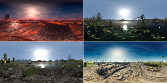
Each topic is carefully researched. Then the 3D artists work to create a scene based on the layout set by the designer. Our main goal is to create a world around the viewer that visually inspires them, and make them understand the context and world which is presented.

Using Blender’s built-in VR rendering features including stereo camera support and equirectangular panoramic camera, we can render the entire scene with one click and deliver the image without stitching or resampling, saving us valuable time.

For VR, the image needs to be noise-free, in stereo, and high resolution. Combining all 3 factors means our rendering time for a 4K by 4K frame is 8 times longer than a traditional 1080p frame. With two consumer-grade GPUs working together (GTX 1070), Cycles was able to crunch through most of our scenes in under 3 hours per frame. The new denoising feature is a huge time saver. Without it, many images can easily take 5x as long to render.

Working in VR has its challenges. Because we are presenting an entire world, not a 2D picture, traditional rules for framing and composition goes out the window. You haven’t designed for VR until “neck comfort” is brought up in a design meeting.

Most of the time, layout also has to use real world scales, this ensures that the stereoscopic effect feels natural. The stereo cameras are placed 6.5cm apart to simulate the human eye separation, and 1.6 meters off the ground to ensure an accurate representation of an average person’s height. Of course, not all scenes take place in the ‘realworld’ scale. Our Expeditions take people into the human body and out to deep space. With these exotic environments, the scale of the world has to be adjusted.

But then, all this hardwork is worth it when we see the reactions from the students:

Lots of oohs and ahs over astronomy in @GuggenheimTch's science classes today thanks to #GoogleExpeditions! #arvrinedu #engage109 #edtech pic.twitter.com/XtJLcgJUie

— Andrea Trudeau (@Andrea_Trudeau)

May 5, 2017

What great reactions as year six explore a volcano! Thank you #googleexpeditions for bringing our learning to life! pic.twitter.com/mAHP2GwLJp

— Stanton_CP (@Stanton_CP)

April 28, 2017

So far, we’ve published over 300 CGI panorama images which can be viewed using  Google Expeditions for Android or Google Expeditions for iOS.

[thepixelary]

Denoising in Cycles for Animation

So many of you wondered how the new denoising feature works in animation. So here is a test:

We rendered this animation using a number of different settings, they are:

100 Samples

100 Samples + Denoising

500 Samples

500 Samples + Denoising

500 Samples + Static Seed

500 Samples + Static Seed + Denoising

1000 Samples

1000 Samples + Static Seed + Denoise

Still Image comparisons

You can watch the video to draw your own conclusion, but here is what we found out:

Denoising is seriously amazing!

At 500 samples, it can turn the animation into something that’s usable.

At 1000 samples, the image is flawless.

To avoid temporal artifact, denoising works best with static seed.

Denoising works well with motionblur, refraction, reflection and depth of field. There are no visisble artifacts.

To get the same image quality without denoising could easily take 8x more samples, that’s 8x the render time.

Without a doubt, this feature brings the greatest performance improvement to Cycles since its inception. You can download the 2.79 test build from https://builder.blender.org/download/ today and try for yourself.

[thepixelary]

Denoising in Cycles Tested

Denoising just landed in Cycles Renderer and it’s far more capable than we ever imagined. Let’s dive in.

Here is a cornell box with 500 samples:

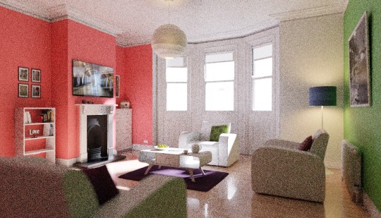
It’s almost not usable at any resolution due to how noisy it is. Let’s render again with denoise using the default settings.

At virtually the same render time, the image is far cleaner than any postprocessing denoiser is capable of. This is because as a builtin denoiser, it’s able to use data from various internal passes to reconstruct a cleaner image.

Just look at how it’s able to pull the detail from the pillow and reconstruct the shape of the teapot!  Sure there are artifacts, but the denoiser is really designed to help you get rid of that last bit of noise. You know, the noise that forces you to render at 10000 samples rather than 3000. The noise that forces you to triples your render time.

So let’s try rendering this scene at a more reasonable sample count of 3000. It’s almost usable, but still noisy.

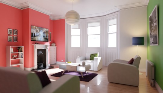
Smooth as butter, and without any visible artifacts.

However, it’s not perfect. We’ve encountered some artifacts even at high sample count when dealing with extremely bright reflection and refractions. Take this scene for example:

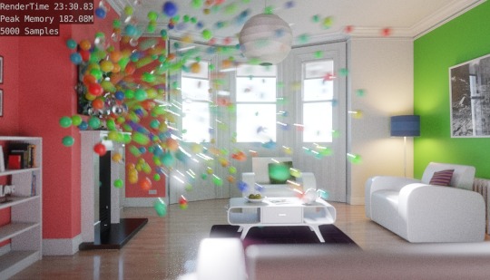
And here is the denoised version:

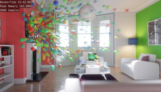
See those black halo artifacts around the balls? They are a result of the denoising filter breaking down at high brightness. A temporary solution is to use clamp direct to limit the brightness of the pixel. This is against our usual recommendation to not touch the clamp value, because it basically defeats the purpose of using a physically realistic pathtracer. But in this case, it’s the only quick way to fix the artifacts. In our case, setting the clamp direct to a high value of 100 is enough to remove the artifact.

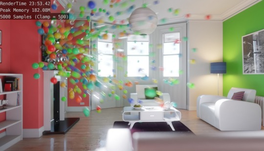
Flawless.

So in summary, we are very excited to see how well the denoising feature is working. It can easily cut down render time by half when used correctly. Check back in a few days to see our results on denoising animations.

[thepixelary]

Filmic Colors in Blender and Light Linearity

By Mike Pan

First of all, a huge thanks to Troy Sobotka, the creator of filmic-blender, for the relentless push to help me understand all of this. This post is a summary of my understanding of color and light as it applies to my work as a CG artist.

From a physics perspective, light and color are inseparable, they are one. You can’t have one without the other. In a pathtracer such as Blender’s Cycles, they are basically the same thing. So I’ll be using these 2 terms interchangeably from now on.

This is going to be a long one, so stay with me. Let’s start by looking at a classic Cornell Box rendering with 1 light source:

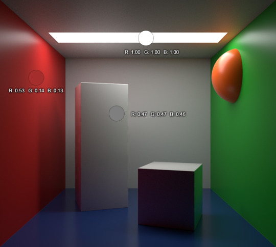
You’ll notice I sampled a few random locations on the image and included their RGB values next to it. We have a red, a grey, and a pure white. So far, so good. Remember, this scene is lit with a single light source from the top. Let’s see what happens when we double the light’s energy from 10 to 20.

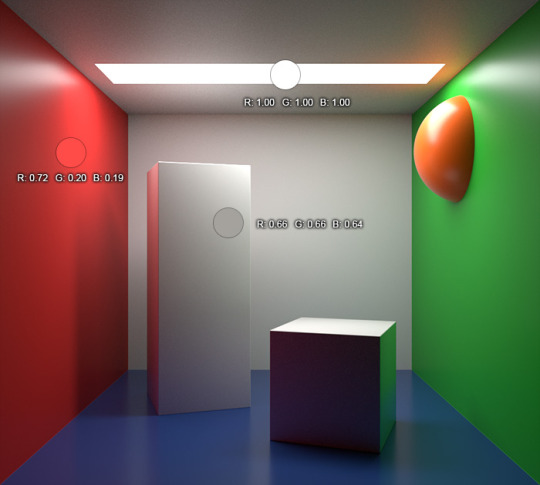
Okay, the overall image got brighter as expected. But if we sample the other 2 locations, we notice something strange. Even though we doubled the intensity of the light, the pixel values didn’t double. Huh.

Let’s look at these previous two images in another way:

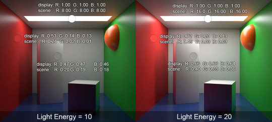
Here I added another row below the first. The ‘display’ value on the top row refers to what we had in the previous images - those are the values as sampled from the JPEG image. The ‘scene’ value is what the rendering engine was actually working with - it represents the light energy level at that pixel. As we can see, even though the display value didn’t double when we doubled the light energy, the scene value indeed doubled as we expected. (They are also not clamped to 1, as evident by the sample on the light panel.

So if the scene values represent the ‘true’ values of the 3D world, why is the final image not showing these values to begin with? And how does the computer transform those scene values to display values?

This is Gamma at work. The history of Gamma is really not important right now. All you should know is the magical value of 2.2. This value is used to transform the scene color into the display color we saw earlier.

Don’t believe me? Raise any scene value to the power of 1/2.2 and you’ll get the corresponding display value.

But why is this transform needed? What does this scene look like if we use the scene color value as-is? In another word, without any transformation?

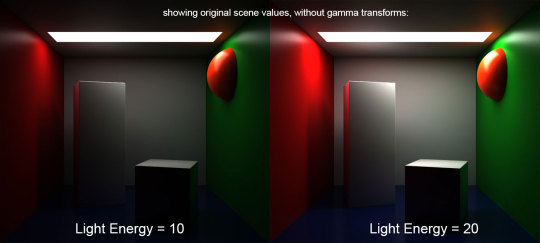
Yuk. Not only is it way too dark, it’s just unpleasant to look at due to the high contrast.

This is the first concept we have to learn today: Scene-referred values and display-referred values are two different things. At the simplest level, we need to apply a gamma transform to the scene-referred color space to get a pleasant looking image in display-referred space.

So now we know how gamma transform is used to change our rendering data into a pleasant looking image, let’s see if there is more we can do to make it look even better. Instead of a simple gamma transform, let’s try to use a look-up-table and that’s designed to give the image a more film-like look, specially the filmic-blender.

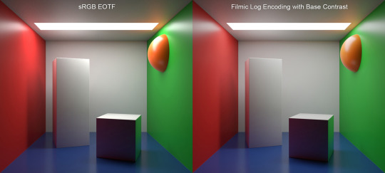
The difference between the original(left) and the filmic version(right) might be subtle. Note the hotspot on the red wall is gone, replaced by a much more natural looking glow. The over-saturated banding on the orange dome is gone too, and its reflection is far less overexposed.  To me, that’s the main benefit of filmic-blender, it is able to show off a much wider dynamic range, and gives the image a much more refined look near over-exposed values, especially on saturated colors.

In summary: The filmic-blender lut is a powerful imaging tool that transforms the linear scene-referred values into nonlinear display-referred values.

But filmic cannot work alone. To really make the most use out of it, the scene has to be lit in a physically accurate way. Cycles is a pathtracing rendering engine, this means for it to work its magic, the lights need to be set to realistic values. Real world has a very wide dynamic range, something that we are not used to in a CG world.

Whenever you are lighting in Cycles, keep in mind that the energy level of the sun lamp is measured in Watts/m². All other lamps use Watts [source]. That means for the most accurate light transport, a single household light bulb should be in the 60-80 range, while the sun should be set to 200-800 for daylight, depending on time of the day, latitude, and cloud cover.

Without proper lighting ratios, your scene will look flat even with filmic lut. Light will not bounce enough, and it will just look artificial. In the image above, the left has a sun set to a low value of 50 because the artists is afraid of blowing out the highlights, but when we set the sun to a more realistic value of 500 as we did on the right, light distribution becomes far more realistic.

Don’t be afraid to let the image blow out. The real world rarely fits within the dynamic range of a camera. The filmic lut is especially helpful in cases with high energy lights, because it’s able to tame those overexposed areas into something that looks far more pleasing. Just compare the room rendered with and without the filmic lut, using the physically correct light ratio:

See all those ugly highlights and super saturated hotspots on the left image? They are gone in the right. Filmic allows you to push your lighting further without worrying about nasty artifacts from overexposure.

So we learned that Filmic is a lut, it transforms your linear scene data into a beautiful nonlinear image. But that doesn’t mean you should use it on every image. Sometimes, you need a linear image to work with.

Let’s talk a bit more about linearity of light.

Light is additive. That means I should be able to separate the contribution of each individual light source and then add them up, to get the exact same image as if all the lights sources are rendered together. The ability to do this, and do this correctly, is crucial for compositing and visual effects where light and color are often adjusted in dramatic ways.

So let’s try that with our room scene. We rendered each light in a separate layer and saved them as 32bit TIFF images:

Huh, that’s didn’t work at all. The combined image is a hot mess.

Even though we saved the individual images as 32bit tiff so the color values are not clamped, the tiff did not record the scene values. When the image is saved, it underwent the scene to display transform, so the values we are seeing is not the linear scene-values, but the nonlinear display-values. This happens regardless if we are using the default sRGB EOFT lut or the Filmic lut.

This is a huge problem because any light or color work manipulation we do is now on a nonlinear dataset that’s not designed to be manipulated in this way. The correct way is to only save and operate on data in a linear format such as EXRs.

Let’s try the same process with EXRs. (Because EXRs are linear, these are mapped to Filmic for display on your screen)

Now everything works exactly as it’s suppose to! Using linear data for compositing is really the only way to ensure that your scene remains physically accurate.

In Blender, all image file formats respect the color management setting(e.g. sRGB or Filmic). Except for EXR, which is always saved in a linear format without any transforms.

Because lights are additive, and we rendered each light of this scene to a separate EXR layer, we can play around with the color and contribution of each light in post and get very different images without any rerendering.

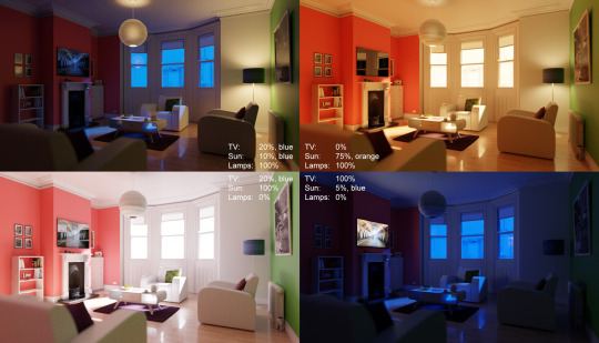
That’s the the flexibility of working with scene-referred data directly. 

So we are finally near the end of this post. There are some simplifications I’ve made in order to make this post more understandable, and there are a lot of issues that I haven’t mentioned. On the color front, we haven’t explored wide gamut and the different color profiles. On the content creation side, there is something to be said about ambient occlusion and clamping and the various compositing nodes that work only on clamped display-referred data(the short version is: don’t use these).

But hopefully this has been a fun but educational journey for you. Stay tuned for Part II.

[thepixelary]

Investigating Cycles Motion Blur Performance

Motion blur in Cycles just got a massive performance improvement in Blender 2.78c. However it’s still a pain to render a large scene with motion blur.  How can we best optimize our render settings? What hardware should we use? We’ve done 18 hours worth of benchmarks on this topic so you don’t have to guess.

All tests are performed on the following system:

Intel i5 2500K @ 4.8Ghz

16GB RAM

2x Nvidia GTX 1070 8GB

Blender 2.78c on Windows 10

But the spec shouldn’t matter since we are looking at relative performance. Let’s start with a simple scene:

Just a bunch of flying bones for a science class. Let’s see how this scene renders with various motion blur length and BVH settings:

Observation:

No motion blur is the fastest. As we increase the shutter speed, performance decreases sightly as the objects gets more smeared. But the overall performance hit of motion blur is negligible.

BVH Time Steps doesn’t affect the performance too much. Probably because there isn’t a lot of intersecting geometry.

Let’s see how this scene does on the GPU:

Observation:

GPU takes a much bigger performance penalty with motion blur than CPU rendering in this scene. But the overall performance is still faster than CPU rendering.

Again, BVH Time Steps doesn’t affect the performance too much.

Okay, let’s bring on a more complex scene! From the Sunny and Gerd short film we worked on. This shot has characters deformations, heavy geometry, and a very fast moving toy specifically setup to stress test the rendering engine:

First, let’s see how CPU tackles this scene:

Ouch, we can really see the performance impact of motion blur in this scene.

Similar to what we observed with the simple scene, the longer the motion blur trail, the slower it is. But the difference is far greater here.

A properly tuned BVH Time Steps can reduce render time substantially, especially on high shutter speed values.

Using a typical shutter speed of 0.5 (which mimics the 180 degree shutter used in movie cameras), we see that motion blur can be rendered at almost the same speed as a non motion blurred scene when BVH Time Steps is set to 3.

BVH Time Steps has a diminishing return, so higher values yields increasingly smaller performance gains.

Before we get too excited, this is how it performs on the GPU:

Yikes.

Performance on the GPU is atrocious as soon as motion blur is turned on.

BVH Time Steps tweaking can keep the render time under control. But it still can’t match the performance without motion blurred.

BVH Time Steps trades off memory in order to speed up the rendering. So higher value will use more memory!

To summarize, tune your BVH Time Steps value! A value of 2 to 3 increases performance significantly on motion blurred scenes. Without it, fast moving objects would be nearly impossible to render. Secondly, CPU performs a lot better with motionblur than GPU.

Sadly, this is only part of the story. Usually for high motionblur scenes, we also have to turn up the number of samples in order to make sure the smear is noise-free. So rendering using motion blur, and expecting the same noise-free image, will require more samples, and therefore take an additional performance hit.

This article is written with Blender 2.78c in mind. The developers of Blender have done an amazing job at improving the performance of Cycles over the years. I am sure it will only get better as time goes on.

[thepixelary]

CPU vs GPU rendering in Blender Cycles

Keeping rendering times under control is something every studio struggles with. As artists, we want to be only limited by our imagination, and not by the computing power we have. At The Pixelary, we are very familiar with the performance characteristics of Cycles. We want to start this blog by sharing some of our knowledge. So let’s dive in and see what offers the best performance and value for cranking out those pixels!

GPU is fast, cheap, and scalable - A $400 gaming GPU like the Geforce GTX 1070 or Radeon RX580 is faster than a 22-core Intel Xeon 2699v4 ($3500) in most renderings tasks. So looking at the price of the hardware alone, GPU is the obvious winner.  The value of GPU is further improved because we can easily put 4 GPUs in a single system and get roughly 4x the speedup, whereas multi-socket CPU systems get really REALLY expensive. But GPUs have one downside...

GPU Memory Limitations - For GPU rendering to work, the Cycles rendering engine need to fit all the scene data into GPU memory,  scenes that don’t fit will simply refuse to render. Most consumer GPUs have 8GB of memory today, this means you will be only able to fit 32 unique 8k textures before you are out of memory - That’s not a lot of textures. GPUs with larger memory capacity do exist, but their price is often astronomical, making GPU rendering as expensive as CPU.  On the other hand, while CPU rendering doesn’t use any less memory, RAM is much cheaper. 32GB of system memory can be purchased at a very reasonable price.

Power Usage - For studios doing a lot of rendering, power consumption is another aspect to consider. Surprisingly, despite the large price difference in price between CPU and GPU, performance per watt is strikingly similar for high-core count devices. A GTX 1070 and a Xeon 2699v4 both have a peak power consumption of about 150W, and performs roughly the same. So regardless of what device you are rendering, hardware of the same generation should use similar amount of power. However, low-core count, high frequency CPUs such as the Intel 7700k tend to draw more power compare to a high-core count, low frequency CPU.

Feature Set - Okay, enough about hardware. We also need to compare the differences in capabilities between CPU and GPU rendering. As of Blender 2.78c, GPU rendering and CPU rendering are almost at feature parity. There are only a small set of features that’s not supported on the GPU, the biggest missing feature being Open Shading Language.  But, unless you are planning to write your own shaders, GPU is as good as the CPU.

Operating Systems - Some people say certain operating systems and compiler renderings up to 20% faster. Wouldn’t that be great if it were true? It’s something we’d like to get to the bottom of. So, we will investigate this claim at a later date and post our findings.

As a small independent studio, GPU rendering makes the most sense because it allows our artists to work fast without breaking the bank.

What about you? What do you think is the best platform for rendering?

[thepixelary]

The Road Ahead

Say hi to the Pixelary! We are a newly established computer animation studio based in Vancouver, Canada.

We believe in transparency - this is our way of giving back to the community. So whenever possible, we will use this space to share what we are doing, the challenges we face, and the results of our labor.

Stay Tuned!