themathlab

[themathlab]

Arithmetic vs. Geometric Sequences

Arithmetic: common adding/subtracting between terms

Geometric: common multiplication between terms

The common difference between terms in a series must be consistent, if not it doesn’t classify as an arithmetic or geometric sequence.

[themathlab]

Arithmetic Series

A series is the terms of the sequence added together to get the full/total value.

[themathlab]

Recursive: A recursive process requires the use of the previous term in a sequence. You NEED to know the term before to figure out the next term. Remember programming: the x & y coordinates needed to know their last coordinates to go on with the program.

Explicit: You can be all like “Damn, I wanna find out how much this plant, is gonna ripen in 45 days if it grows consistently 3 cm.” Then you can be all like, well imma use a explicit function cause its repetitive asf.

A recursive process requires the calculation of each term as each term relies on the term before it.

An explicit equation allows the calculation of any term in the sequence.

Variables:

“n”: position in the sequence

“d”: common difference

[themathlab]

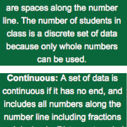
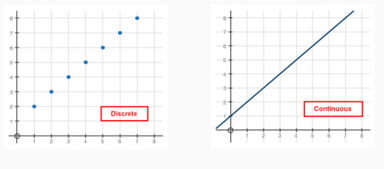
Discrete Vs. Continuous Data Sets

You cannot draw a curve or line on the graphs of discrete sets of data. That is why there is spaces along the number line.

Continuous: yes you can draw a curve or line because it includes all the numbers along the curve or line.

[themathlab]

Arithmetic Sequences

An arithmetic sequence is a list of numbers, called terms, which share a common difference.

Needs to be a consistent difference.

3 Steps to Derive the Arithmetic Function

Know first term of sequence

Find the common difference between the terms.

Keep multiplying common difference to the current position of the term (1st, 2nd, 3rd, etc) minus 1.

Formula:

First Term + (Current Position in the sequence minus 1)●(common difference)

Domain(position in set): all natural numbers (numbers greater than or equal to 1) Makes sense because you have 1st, 2nd, 3rd, etc. Starts with 1st place/position)

Range: Freedom to do whatever the fck you want

Variables

an = a1 + (n − 1)d

a1 is the first term of the sequence

n is the position number of a given term

d is the common difference between the terms

an is the value of the term in the given position number.

[themathlab]

Limitations of Synthetic Division

Synthetic division and long division are two valid methods for dividing polynomials; however, make note of some limitations that exist.

To use synthetic division,

the divisor must be a BINOMIAL of degree ONE. (If the divisor is a monomial, trinomial, or polynomial, synthetic division will not work).

Leading coefficient must be ONE.

if the highest exponent or leading coefficient of the binomial is anything other than one (such as x3 − 2 or 5x+ 4), synthetic division cannot be applied.

[themathlab]

Behavior of Graphs

Note: if exponent is odd, graph will haves ends that continue in opposite directions.

If exponent is even, graph will have ends that continue in same direction.

[themathlab]

Shifting Functions

f(x + c) : horizontal shift (left or right) the function is moved “c” units;

(x+c) = left

(x-c) right

f(x) + c : vertical shift (up or down)

f(x) + c = up

f(x) - c = down

f(cx) : affects the shape of the graph

c > 1 = narrow

c < 1 = widens

c is negative (-) = opens down

c ● f(x) : whole function is multiplied by “c” so it can affect it in all the ways previously mentioned

[themathlab]

Graphing a Parabola

Find the axis of symmetry (x-coordinate of vertex)

Substitute x-coordinate of vertex into function

The answer of this substitution will result in y-coordinate of vertex

Randomly select x-coordinates on either side of the vertex (if vertex is 2 (for example) select [0,1 or 3,4]

Substitute the randomly selected x-coordinates into the function to find the corresponding y-coordinate so you can plot the point.

Graph the points and connect them w/ a parabola.

[themathlab]

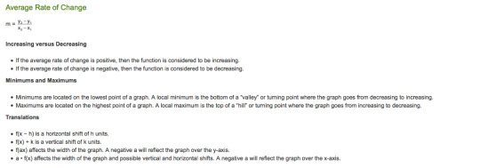
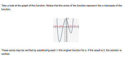
Keys Features of Polynomial Graphs

Average Rate of Change

Minimums and Maximums

Translations or Shifting Functions

[themathlab]

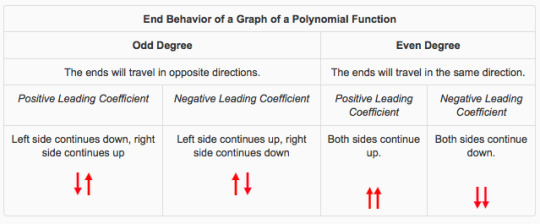
End Behavior of a Graph of a Polynomial Function

When the degree of a function is an odd number, it can be said that the ends of the graph continue in opposite directions. One end goes up while the other goes down.

When the degree of a function is an even number, the ends of the graph point in the same direction. Both ends go up or both ends go down.

[themathlab]

Solving Polynomial Equations

1. Find out how many possible zeros you can have by looking at the degree of the function.

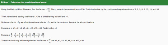
2. Use the Rational Root Theorem to find the factors of p/q. These factors will be synthetically divided by the function to find the zeros.

P: constant term at the end of the equation

Q: leading coefficient of the 1st term

Get the factors of p & write them over as a fraction with the factors of Q as the denominator

Account for all of the different combinations

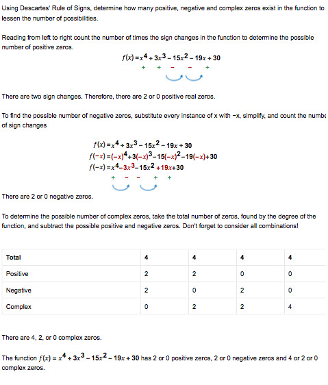
3. Use Descartes’ Rule of Signs

Count sign changes to find positive/negative/complex zeros

For negative zeros, substitute “-x” in the original function

For complex zeros just subtract the number of positive and negative zeros to find how many complex zeros.

4. Using Fundamental Theorem of Algebra

Make a chart stating all the possible combinations of zeros.

This makes it easier when testing the factors. If you only have 1 positive real zero and you find one positive real zero when plugging n the factors, then you don’t have to keep solving for positive real zeros. Move onto negative zeros. This strategy saves time.

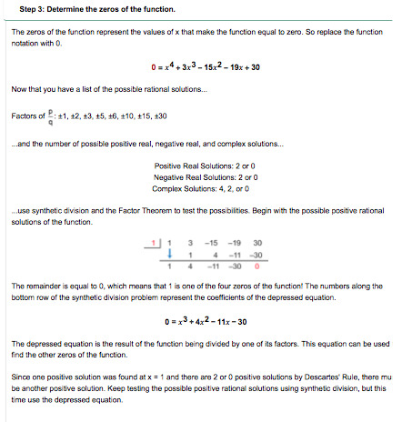
5. Test the factors

Plug in all the factors from Step 2 of the Rational Root Theorem

Shortcut: always check your chart from Step 4.

Don’t keep solving if you’ve found the specified amount of zeros per column.

You know its a factor if you use the factor as the divisor in a problem where you are synthetically dividing the function by the factor.

Remainder is zero? It’s a factor!

6. Depressed Equation

Found a factor where the remainder is zero? Awesome.

Now you can use the quotient produced by the synthetic division of the function and the possible factor.

To get the degree of the depressed equation, subtract “1″ from the original degree.

This depressed equation (if it has a degree of 2/quadratic) can be used to find the remaining zeros of the function.

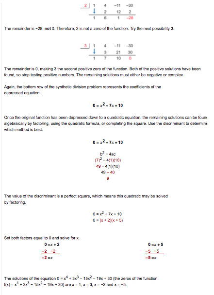
7. Find the Zeros

Look at the depressed equation to find the remaining zeros. They may even be complex.

Note: If you are solving for zeros and you can’t find them, then they might be irrational. Ewe.

8. Substitute the zeros of the function into the equation.

If they are true zeros, then the answer will always be zero.

[themathlab]

Solving Polynomial Equations

[themathlab]

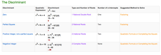
The Discriminant

Figure out which method of factoring you should use and why

[themathlab]

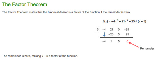
Factor Theorem

If you divide something, and the remainder is zero, then it is a factor.

[themathlab]

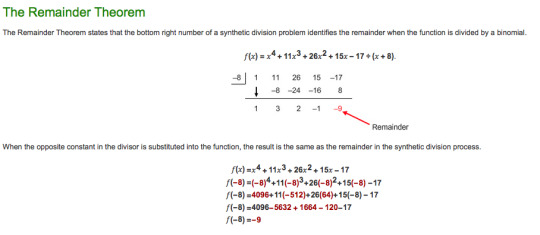
The Remainder Theorem

You can find the remainder of a polynomial division problem by getting the opposite value of the divisor’s constant (if positive, turn negative. if negative, turn positive) and plugging it into the dividend’s function.

[themathlab]

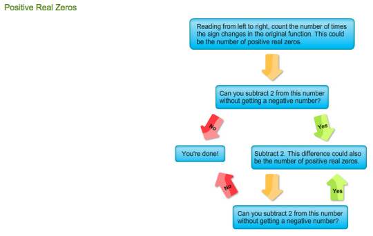
Using Descartes Rule of Signs:

1. Find the Positive Zeros

Count how many times the sign changes between terms.

The # of times the sign changes between terms is the # of positive real zeros.

Subtract 2 from this number. If the number is not negative, then that is another number amount of positive real zeros.

Usually 2 values for the amount of positive real zeros. They are added to a chart and you must take into account all of the different combinations.

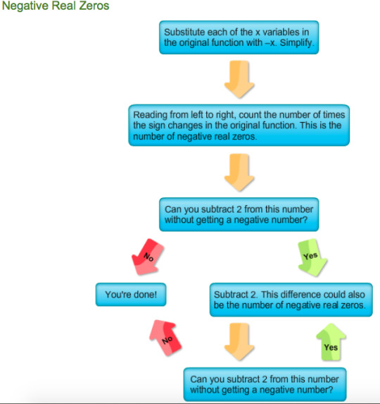
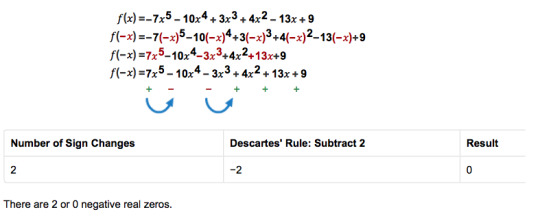
2. Find the Negative Zeros

Substitute each of the values of “x” in the original function with “-x”. Distribute and simplify.

Count the number of times the sign changes between terms.

This is the number of negative real zeros.

Subtract 2 from this number. If the number is not negative, then that is another number amount of negative real zeros.

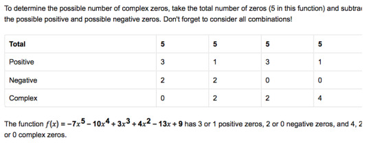
3. Find the Complex Zeros

Make a chart documenting the possible numbers of positive and negative real zeros. There are different combinations because when you subtract 2 from the number of sign changes you get, that answer is another possible amount of zeros.

Add up the possible amount of positive and negative real zeros (of its specific column) and subtract it from the degree of the polynomial.

Voila! That is your number of complex zeros.