#smfs bracket

[takethistoyourstardust]

oh god the next bridge bracket is gonna be smfs vs crashing, and the winner of that is gonna go up against bkt... evil evil EVIL bracket

[so-much-for-stardust-bracket]

reblogs appreciated :)

[icecreamheadachez]

Give it a couple of days to settle, rn i'm seeing a bunch of "favourite song from smfs" posts, filled with people yelling they can't decide, and exactly one that was more nuanced and asked which one was more of a bop, but in a few days with the album better processed and when people aren't making the same poll over and over a smfs song-off would be cool. Also waiting a couple of days to see what consensus seems to be in which songs have similar vibes or have appealed most as bops/soul destruction will help with seeding the matchups if you do it in a bracket competition style.

ur 100% right!!! i'll need some time to listen more myself and also cus i've never rlly done a bracket competition before so i'll have to plan it out n stuff :D

[marindani11-blog]

K-MEANS CLUSTER ANALYSIS

DATA MANAGEMENT

For this week’s assignment I ran a k-mean cluster analysis to identify subgroups of adolescents based on 14 variables representing (gender) Male; (race/ethnicity) Hispanic, White, Black, Native American and Asian; (parent’s education level) mother’s level of education and father’s level of education; (extracurricular activities) time spent watching tv, time spent in sports and whether the student has a job; Use of other drugs and (academic behavior) grades and years expelled from school. All clustering variables were standardized to have a mean of 0 and standard deviation of 1.

MODEL

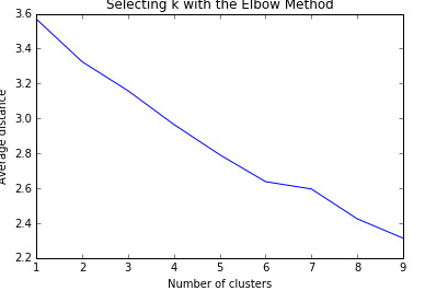
I specified k = 1 to 9 clusters and a series of k-means cluster analyses were conducted using Euclidean distance. The variance in the clustering variables was plotted for each of the cluster solutions (1 to 9) in an elbow curve to provide guidance for choosing the number of clusters to interpret.

The results could be interpreted of a 6-cluster solution. Thus, I ran the analysis again limiting k to 6. I plotted the first two canonical variables for the clustering variables by cluster (represented by color).

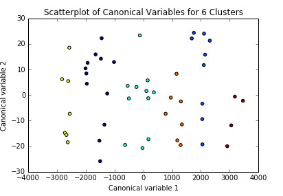
Initially, we can think the clusters are well represented since they don’t seem to be overlapping.  I analyzed it further by comparing the means on the clustering variables, compared to other clusters.

Following up, I tested the validity of the clusters with an analysis of variance (ANOVA). I tested for significant differences between the clusters on violence levels (measured as the number of times the person was in a fight during the past year). A tukey test was used for post hoc comparisons between the clusters. Results indicated significant differences between the clusters on violence ( p<.0001). The tukey post hoc comparisons, however did not showed significant differences between clusters on violence levels,  with the exception that clusters 1 and 2 that were significantly different from each other.

Adolescents in cluster 1 had the highest violence levels (mean=3,84, sd=0.4), and cluster 2 had the lowest violence levels (mean=0.2, sd=0.7). In cluster 1 we have the group of adolescents with the lowest parental level of education (for both parents) and the highest probability of being expelled from school. 

CODE

@author: marindani11 """ import pandas as pd from pandas import Series from pandas import DataFrame import numpy as np import matplotlib.pylab as plt import pickle from sklearn.cross_validation import train_test_split from sklearn import preprocessing from sklearn.cluster import KMeans from scipy.spatial.distance import cdist from sklearn.decomposition import PCA import statsmodels.formula.api as smf import statsmodels.stats.multicomp as multi

#IMPORT DATA PREVIOUSLY CLEANED FOR THIS EXCERCISE with open('decisionTree.pickle', 'rb') as data:    dataset = pickle.load(data)

#DATA MANAGEMENT #Create 2 data sets: 1 includes only the predictor variables, # 2 includes the response variable recode1 = {1:1, 2:0} dataset['MALE']= dataset['BIO_SEX'].map(recode1)

#violence dataset['VIOLENCE']=dataset['H1FV13'].convert_objects(convert_numeric=True) dataset['VIOLENCE'] = dataset['VIOLENCE'].replace([996,997,998,999], np.nan) dataset['VIOLENCE']=dataset['VIOLENCE'].dropna()

#Marijuana Use over lifetime dataset['MJUSE']=dataset['H1TO33'].convert_objects(convert_numeric=True) dataset['MJUSE'] = dataset['MJUSE'].replace([996,997,998,999], np.nan) dataset['MJUSE']=dataset['MJUSE'].dropna()

#Alcohol Use over past year dataset['ALCOHOLUSE']=dataset['H1TO16'].convert_objects(convert_numeric=True) dataset['ALCOHOLUSE'] = dataset['ALCOHOLUSE'].replace([996,997,998,999], np.nan) dataset['ALCOHOLUSE']=dataset['ALCOHOLUSE'].dropna()

#Expelled from school dataset['EXPELLED']=dataset['H1ED9'].convert_objects(convert_numeric=True) dataset['EXPELLED']=dataset['EXPELLED'].replace([6,8], np.nan) dataset['EXPELLED']=dataset['EXPELLED'].dropna()

#Clean the dataset dataset=dataset.dropna()

#SELECT PREDICTORS cluster=dataset[['LATINOS', 'WHITE','BLACK','AMINDIAN','ASIAN','MOTHEREDU', 'FATHEREDU','TVTIME','SPORTSTIME','JOB','MJUSE','MALE','EXPELLED','GRADES']]

cluster.describe()

#Predictors need to be standardize so they're comparable. #Standardization of mean = 0; standard deviation= 1 #dataset=dataset.dropna() clustervar=cluster.copy() "the preprocessing.scale function transform the variable into one with mean 0 and stdv 1" "float64 ensures the variables have a numeric format" clustervar['LATINOS']=preprocessing.scale(clustervar['LATINOS'].astype('float64')) clustervar['WHITE']=preprocessing.scale(clustervar['WHITE'].astype('float64')) clustervar['BLACK']=preprocessing.scale(clustervar['BLACK'].astype('float64')) clustervar['AMINDIAN']=preprocessing.scale(clustervar['AMINDIAN'].astype('float64')) clustervar['ASIAN']=preprocessing.scale(clustervar['ASIAN'].astype('float64')) clustervar['MOTHEREDU']=preprocessing.scale(clustervar['MOTHEREDU'].astype('float64')) clustervar['FATHEREDU']=preprocessing.scale(clustervar['FATHEREDU'].astype('float64')) clustervar['TVTIME']=preprocessing.scale(clustervar['TVTIME'].astype('float64')) clustervar['SPORTSTIME']=preprocessing.scale(clustervar['SPORTSTIME'].astype('float64')) clustervar['JOB']=preprocessing.scale(clustervar['JOB'].astype('float64')) clustervar['MJUSE']=preprocessing.scale(clustervar['MJUSE'].astype('float64')) clustervar['MALE']=preprocessing.scale(clustervar['MALE'].astype('float64')) clustervar['EXPELLED']=preprocessing.scale(clustervar['EXPELLED'].astype('float64')) #clustervar['PARENTALCTRL']=preprocessing.scale(clustervar['PARENTALCTRL'].astype('float64')) #clustervar['COCAINEUSE']=preprocessing.scale(clustervar['COCAINEUSE'].astype('float64')) clustervar['GRADES']=preprocessing.scale(clustervar['GRADES'].astype('float64'))

# split data into train and test sets clus_train, clus_test = train_test_split(clustervar, test_size=.3, random_state=123) "random datasets with 70%/30% of the data"

#MODEL # k-means cluster analysis "we don't know how many clusters may be optimal, so we create an array of numbers between 1 and 10" clusters= range(1,10) "this will give us the cluster solutions for k=1 and k=9 when we test it" meandist=[] "it will be use to store the average distance values that will calculate for each k 1 to 9"

for k in clusters:    model=KMeans(n_clusters=k)    model.fit(clus_train)    clusassign=model.predict(clus_train)    meandist.append(sum(np.min(cdist(clus_train,model.cluster_centers_, 'euclidean'),axis=1))/clus_train.shape[0]) "for each value of k between 1 to 9,n_clusters indicates the # of clusters" "clusassign stores, for each observation, the cluster number to which it was assigned based on the cluster analysis" "model.predict is use to store the closest cluster that each observation belongs to." "then we calculate the average distance between each observation and the cluster centeroids." "we use the np.min function to calculate the smallest (minimum) difference for each observation among cluster centroids" "then we use the sum function to sum the minimum distances across all observations." "he / clus_train.shape with 0 in brackets divides the sum of the distances by the number of observations in the " "clus_train data set where the .shape with 0 in brackets code returns the number of observations in the clus_train data set."

#VISUALIZATION # plot average distance from observations from the cluster centroid "we use the Elbow Method to identify number of clusters to choose." plt.plot(clusters,meandist) plt.xlabel('Number of clusters') plt.ylabel('Average distance') plt.title('Selecting k with the Elbow Method')

#We saw the bend in cluster #8, so we'll re run the analysis model6=KMeans(n_clusters=6) model6.fit(clus_train) clausassign=model6.predict(clus_train)

"use canonical discriminant analysis that creates smaller number of variables, so we can plot in a p dimension" pca_2=PCA(2) "returns 2 best canonical variables" plot_columns=pca_2.fit_transform(clus_train) "asks python to fit the clusters into canonical variables" plt.scatter(x=plot_columns[:,0],y=plot_columns[:,1], c=model6.labels_,) plt.xlabel('Canonical variable 1') plt.ylabel('Canonical variable 2') plt.title('Scatterplot of Canonical Variables for 6 Clusters') plt.show()

#Pattern of means on the clustering variables for each cluster to see whether they are distinct and meaningful "create a unique identifier variable for clus train dataset that has the clustering variables" clus_train.reset_index(level=0,inplace=True) cluslist=list(clus_train['index']) labels=list(model6.labels_) "list of the cluster assignment for each observation" "combine both lists into a directory: dict command creates dictionary, zip command combines lists" newlist=dict(zip(cluslist,labels)) "convert the dictionary into a dataframe" newclus=DataFrame.from_dict(newlist,orient='index') "rename the cluster assignment column" newclus.columns=['cluster'] "create a unique identifier for the cluster assignment to merge with cluster training data" newclus.reset_index(level=0, inplace=True) "merge cluster assignment dataframe with cluster training variable datafrem by index variable" merged_train=pd.merge(clus_train,newclus,on='index') "on=index matches them by index" merged_train.head(n=100) "Calculate clustering variables by cluster" clustergrp=merged_train.groupby('cluster').mean() print("Clustering variable means by cluster") print(clustergrp)

#Test clusters with respect of violent behaviour

violence_data=dataset['VIOLENCE'] violence_train, violence_test=train_test_split(violence_data,test_size=.3,random_state=123) violence_train1=pd.DataFrame(violence_train) violence_train1.reset_index(level=0,inplace=True) merged_train_all=pd.merge(violence_train1,merged_train,on='index') sub1=merged_train_all[['VIOLENCE','cluster']].dropna()

#use analysis of variance to see if there are significant differences between clusters on violence levels violmod = smf.ols(formula='VIOLENCE ~ C(cluster)', data=sub1).fit() print (violmod.summary())

print ('means for violence by cluster') m1= sub1.groupby('cluster').mean() print (m1)

print ('standard deviations for violence by cluster') m2= sub1.groupby('cluster').std() print (m2)

#Tukey test to evaluate post hoc comparisons btw clusters using multi comparison function mc1 = multi.MultiComparison(sub1['VIOLENCE'], sub1['cluster']) res1 = mc1.tukeyhsd() print(res1.summary())

[so-much-for-stardust-bracket]

reblogs appreciated :)

[so-much-for-stardust-bracket]

reblogs appreciated :)

[so-much-for-stardust-bracket]

reblogs appreciated :)

[so-much-for-stardust-bracket]

Fall Out Boy's hottest girls qualified for the final round. may the best win.

reblogs appreciated :)

[so-much-for-stardust-bracket]

reblogs appreciated :)

[so-much-for-stardust-bracket]

reblogs appreciated :)

[so-much-for-stardust-bracket]

reblogs appreciated :)

[so-much-for-stardust-bracket]

reblogs appreciated :)

[so-much-for-stardust-bracket]

reblogs appreciated :)

[so-much-for-stardust-bracket]

hello people✨✨

i will make a smfs song bracket. i hope you all have fun voting!