#sffamily
Explore tagged Tumblr posts
Visit Tumblr Blog
Explore Tumblr blogs with no restrictions, modern design and the best experience.
Last Seen Tumblr Blogs


Fun Fact
Tumblr has a low social media market share in South America.
Photo

#unonight #sffamily (at ตลาดนัดเลียบด่วน รามอินทรา) https://www.instagram.com/p/ClJfd0ghhkW/?igshid=NGJjMDIxMWI=
0 notes
Photo

Celebration meal #SFfamily❤️ https://www.instagram.com/p/BunM_mXhVY7/?utm_source=ig_tumblr_share&igshid=1p0apnq3pd1k1
0 notes
Photo

Stay tuned: We will tell you all about our new #cardgame tomorrow Fogust 1st 🌁 . . #sanfrancisco #sflandmarks #haightashbury #castro #chinatown #unionsquare #lombardstreet #goldengatebridge #SF #🌁 #preview #sftravel #sfsightseeing #fogaholics #foglife #fogust #onlyinsf #digitalpainting #kickstarter #illustration #kidsgames #sffamily #sfmom #familygame #unplugandplay #jogojoy #sfetsy (at San Francisco, California) https://www.instagram.com/p/Bl6VGF5lg7i/?utm_source=ig_tumblr_share&igshid=18m4n6qzzc2h4
#sfetsy#sftravel#onlyinsf#digitalpainting#kickstarter#sf#unionsquare#fogaholics#sanfrancisco#sflandmarks#cardgame#🌁#fogust#sfmom#preview#haightashbury#lombardstreet#unplugandplay#sffamily#familygame#chinatown#kidsgames#foglife#illustration#castro#goldengatebridge#jogojoy#sfsightseeing
0 notes
Text
\documentclass{beamer}
\usepackage[utf8]{inputenc}
\usepackage[english, russian]{babel} % Russian layout
\usepackage{amsmath,mathrsfs,amsfonts,amssymb}
\usepackage[demo]{graphicx}
\usepackage{epic,ecltree}
\usepackage{verbatim}
\usepackage{mathtext}
\usepackage{fancybox}
\usepackage{multirow}
\usepackage{fancyhdr}
\usepackage{enumerate}
\usepackage{epstopdf}
\usepackage{amsmath}
\usepackage{blindtext}
\usepackage{scrextend}
\usepackage{mathtools}
\usepackage[T1]{fontenc}
\usepackage{textcomp}
\usepackage{siunitx}
\usepackage[noend]{algorithmic}
\usepackage{graphicx}
\usepackage{cleveref}
\usepackage{hyperref}
\usepackage{amsmath}
\usepackage{lineno}
\usepackage{caption}
\usepackage{subcaption}
\geometry{paperwidth=140mm,paperheight=105mm}
%\usepackage{bibentry} %for nonbibliography
\usepackage{comment}
\usepackage{color}
\usepackage{caption}
\captionsetup[figure]{labelformat=empty}
\captionsetup[table]{labelformat=empty}
\renewcommand{\thesubfigure}{\asbuk{subfigure}}
\newcommand{\X}{{\mathbf{X}}}
\newcommand{\w}{{\mathbf{w}}}
\newcommand{\A}{{\mathbf{A}}}
\newcommand{\xx}{{\mathbf{x}}}
\newcommand{\y}{{\mathbf{y}}}
\newcommand{\Hm}{{\mathbf{H}}}
\newcommand{\Wj}{\mathbf{W}_j}
\newcommand{\x}{\mathbf{x}}
\newcommand{\bx}{\mathbf{x}}
\newcommand{\bw}{\mathbf{w}}
\newcommand{\by}{\mathbf{y}}
\newcommand{\bb}{\mathbf{b}}
\newcommand{\bnu}{\mathbf{\nu}}
\newcommand{\bX}{\mathbf{X}}
\newcommand{\bY}{\mathbf{Y}}
\newcommand{\bA}{\mathbf{A}}
\newcommand{\bU}{\mathbf{U}}
\newcommand{\bV}{\mathbf{V}}
\newcommand{\bS}{\mathbf{S}}
\newcommand{\bQ}{\mathbf{Q}}
\newcommand{\bI}{\mathbf{I}}
\newcommand{\bbR}{\mathbb{R}}
\newcommand{\bchi}{\boldsymbol{\chi}}
\newcommand{\calC}{\mathcal{C}}
\newcommand{\caligc}{\mathcal{c}}
\newcommand{\calP}{\mathcal{P}}
\newcommand{\calR}{\mathcal{R}}
\newcommand{\calJ}{\mathcal{J}}
\newcommand{\calI}{\mathcal{I}}
\newcommand{\calA}{\mathcal{A}}
\newcommand{\calL}{\mathcal{L}}
\newcommand{\frakD}{\mathfrak{D}}
\newcommand{\frakM}{\mathfrak{M}}
\newcommand{\frakL}{\mathfrak{L}}
\newcommand{\frakC}{\mathfrak{C}}
\newcommand{\frakm}{\mathfrak{m}}
\newcommand{\vif}{\mathrm{VIF}}
\newcommand{\rss}{\mathrm{RSS}}
\newcommand{\tss}{\mathrm{TSS}}
\newcommand{\bic}{\mathrm{BIC}}
\newcommand{\radj}{R_{\text{adj}}^2}
\newcommand{\inter}{\text{int}}
\newcommand{\exter}{\text{ext}}
\newcommand{\T}{{\text{\tiny\sffamily\upshape\mdseries T}}}
\newcommand{\argmin}{\mathop{\arg \min}\limits}
\newcommand{\argmax}{\mathop{\arg \max}\limits}
\usetheme{Warsaw}%{Singapore}%{Warsaw}%{Warsaw}%{Darmstadt}
\usecolortheme{sidebartab}
\setbeamercolor{structure}{fg=white!10!black}
\usepackage{biblatex}
\addbibresource{references.bib}
\setbeamertemplate{bibliography item}[text]
\date{}
\title{04.01.2017}
% A subtitle is optional and this may be deleted
\subtitle{Vector LBP with aggregation via DD: results}
\author{Gorodnitskii Oleg: o.gorodnitskii@skoltech.ru}
\AtBeginSubsection[GaBP preconditioned conjugate gradient method]
{
\begin{frame}<beamer>{Outline}
\tableofcontents[currentsection,currentsubsection]
\end{frame}
}
%----------------------------------------------------------------------------------------------------------
\begin{document}
\begin{frame}
\titlepage
\end{frame}
\begin{frame}{Short description:}
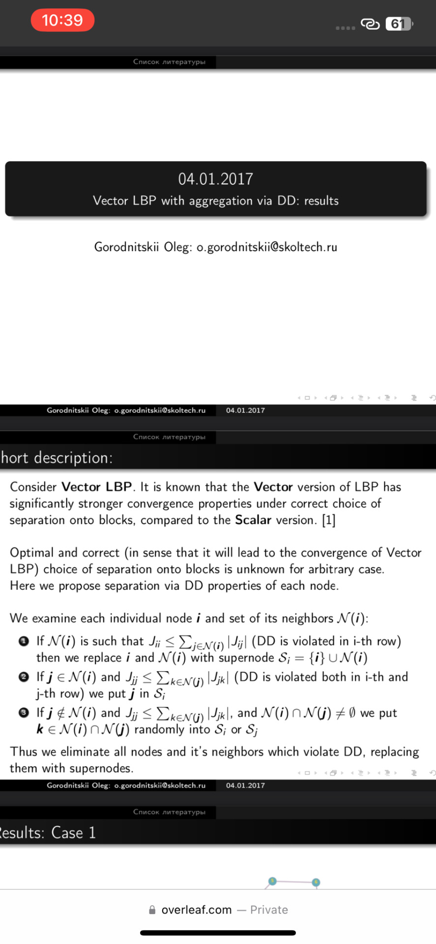
Consider \textbf{Vector LBP}. It is known that the \textbf{Vector} version of LBP has significantly stronger convergence properties under correct choice of separation onto blocks, compared to the \textbf{Scalar} version. \cite{mal08}\\
Optimal and correct (in sense that it will lead to the convergence of Vector LBP) choice of separation onto blocks is unknown for arbitrary case.\\
Here we propose separation via DD properties of each node.\\
We examine each individual node $\pmb{i}$ and set of its neighbors $\mathcal{N}(\pmb{i})$:
\begin{enumerate}
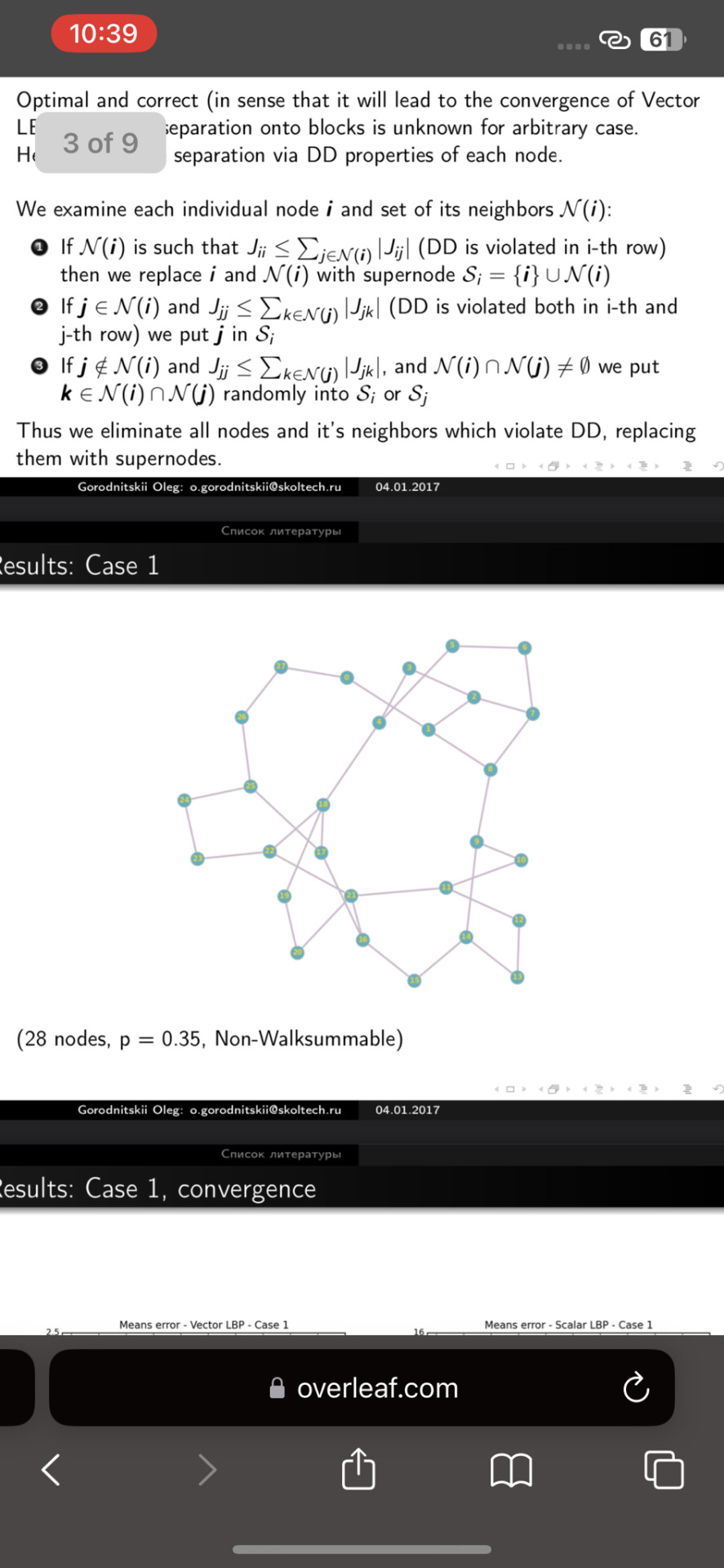
\item If $\mathcal{N}(\pmb{i})$ is such that $J_{ii} \leq \sum_{j \in \mathcal{N}(\pmb{i})}|J_{ij}|$ (DD is violated in i-th row) then we replace $\pmb{i}$ and $\mathcal{N}(\pmb{i})$ with supernode $\mathcal{S}_i = \{\pmb{i}\} \cup \mathcal{N}(\pmb{i})$
\item If $\pmb{j} \in \mathcal{N}(\pmb{i})$ and $J_{jj} \leq \sum_{k \in \mathcal{N}(\pmb{j})}|J_{jk}|$ (DD is violated both in i-th and j-th row) we put $\pmb{j}$ in $\mathcal{S}_i$
\item If $\pmb{j} \notin \mathcal{N}(\pmb{i})$ and $J_{jj} \leq \sum_{k \in \mathcal{N}(\pmb{j})}|J_{jk}|$, and $\mathcal{N}(\pmb{i}) \cap \mathcal{N}(\pmb{j}) \neq \emptyset$ we put $\pmb{k} \in \mathcal{N}(\pmb{i}) \cap \mathcal{N}(\pmb{j}) $ randomly into $\mathcal{S}_i$ or $\mathcal{S}_j$
\end{enumerate}\\
Thus we eliminate all nodes and it's neighbors which violate DD, replacing them with supernodes.
\end{frame}
%-----------------------------------------------------------------------------------------------------
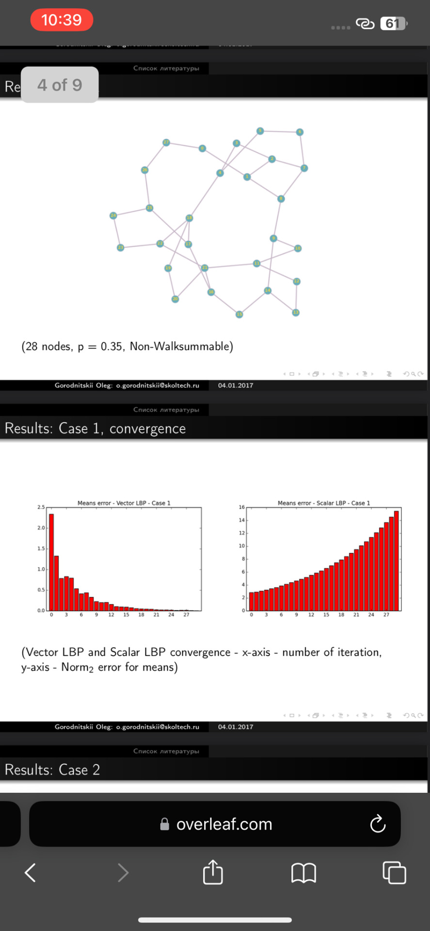
\begin{frame}{Results: Case 1}
\begin{center}
\includegraphics[scale = 0.35]{graph_1}
\end{center} (28 nodes, p = 0.35, Non-Walksummable)\\
\end{frame}
%-----------------------------------------------------------------------------------------------------
\begin{frame}{Results: Case 1, convergence}
\begin{center}
\includegraphics[scale = 0.42]{Means_err_vec_1}
\includegraphics[scale = 0.42]{Means_err_scalar_1}
\end{center} (Vector LBP and Scalar LBP convergence - x-axis - number of iteration, y-axis - $\text{Norm}_2$ error for means)\\
\end{frame}
%-----------------------------------------------------------------------------------------------------
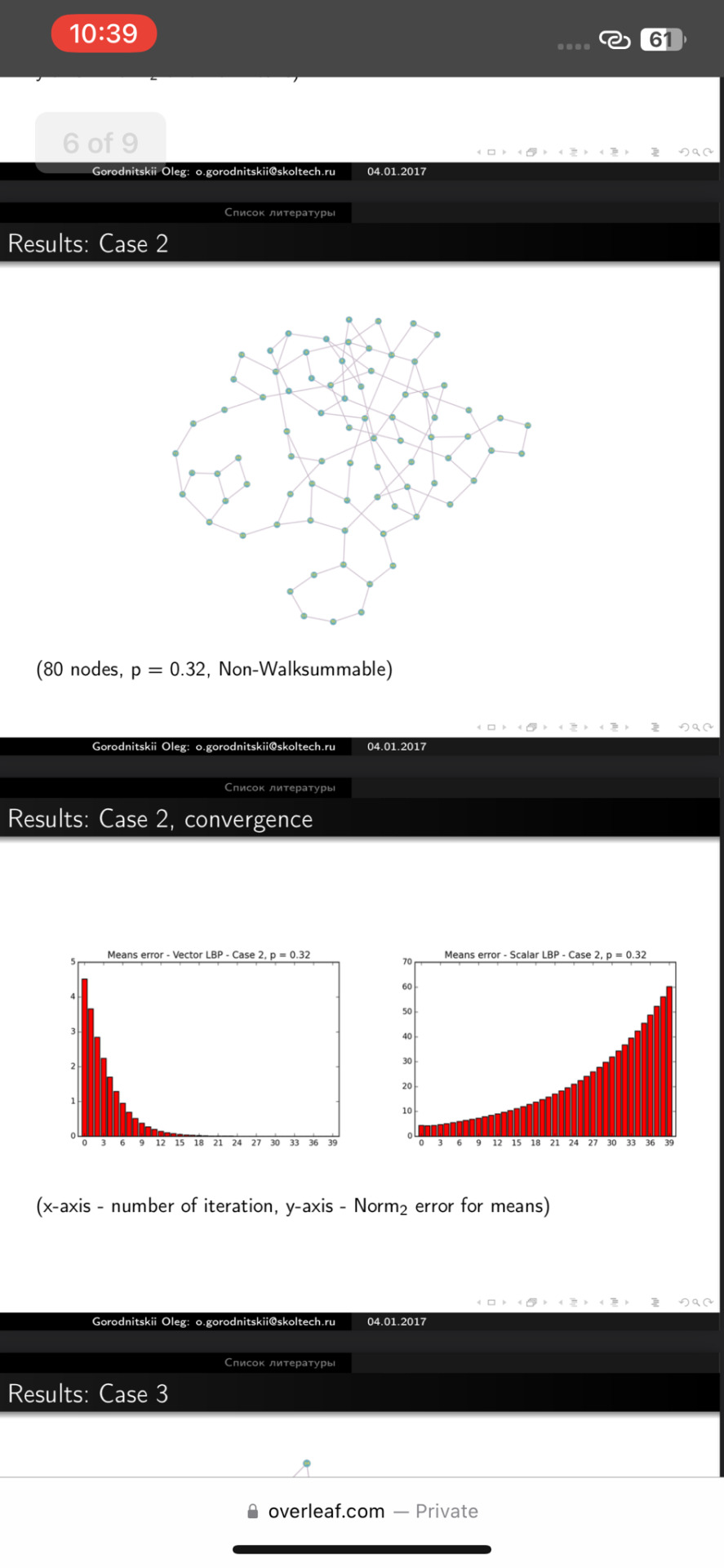
\begin{frame}{Results: Case 2}
\begin{center}
\includegraphics[scale = 0.33]{graph_2}
\end{center} (80 nodes, p = 0.32, Non-Walksummable)\\
\end{frame}
%-----------------------------------------------------------------------------------------------------
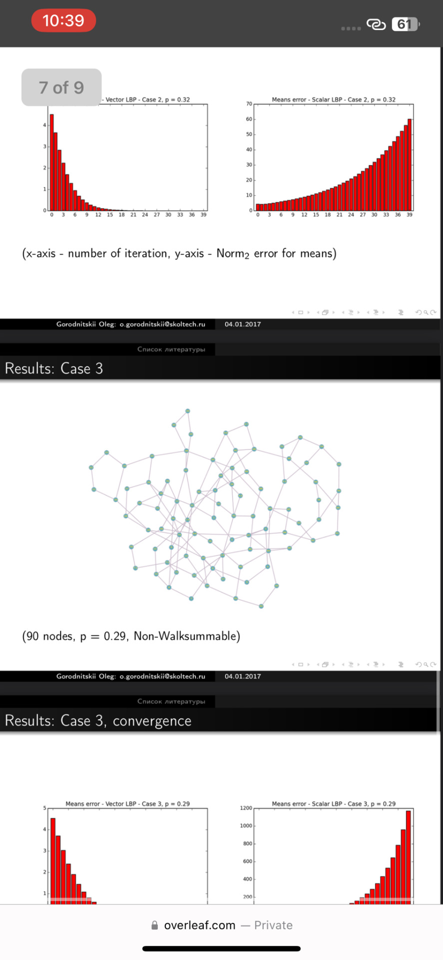
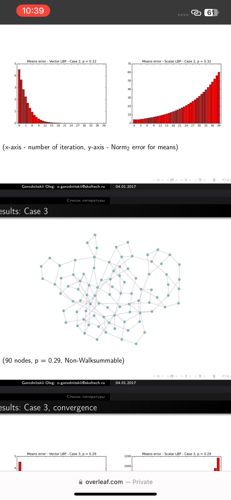
\begin{frame}{Results: Case 2, convergence}
\begin{center}
\includegraphics[scale = 0.42]{Means_err_vec_2}
\includegraphics[scale = 0.42]{Means_err_scalar_2}
\end{center} (x-axis - number of iteration, y-axis - $\text{Norm}_2$ error for means)\\
\end{frame}
%-----------------------------------------------------------------------------------------------------
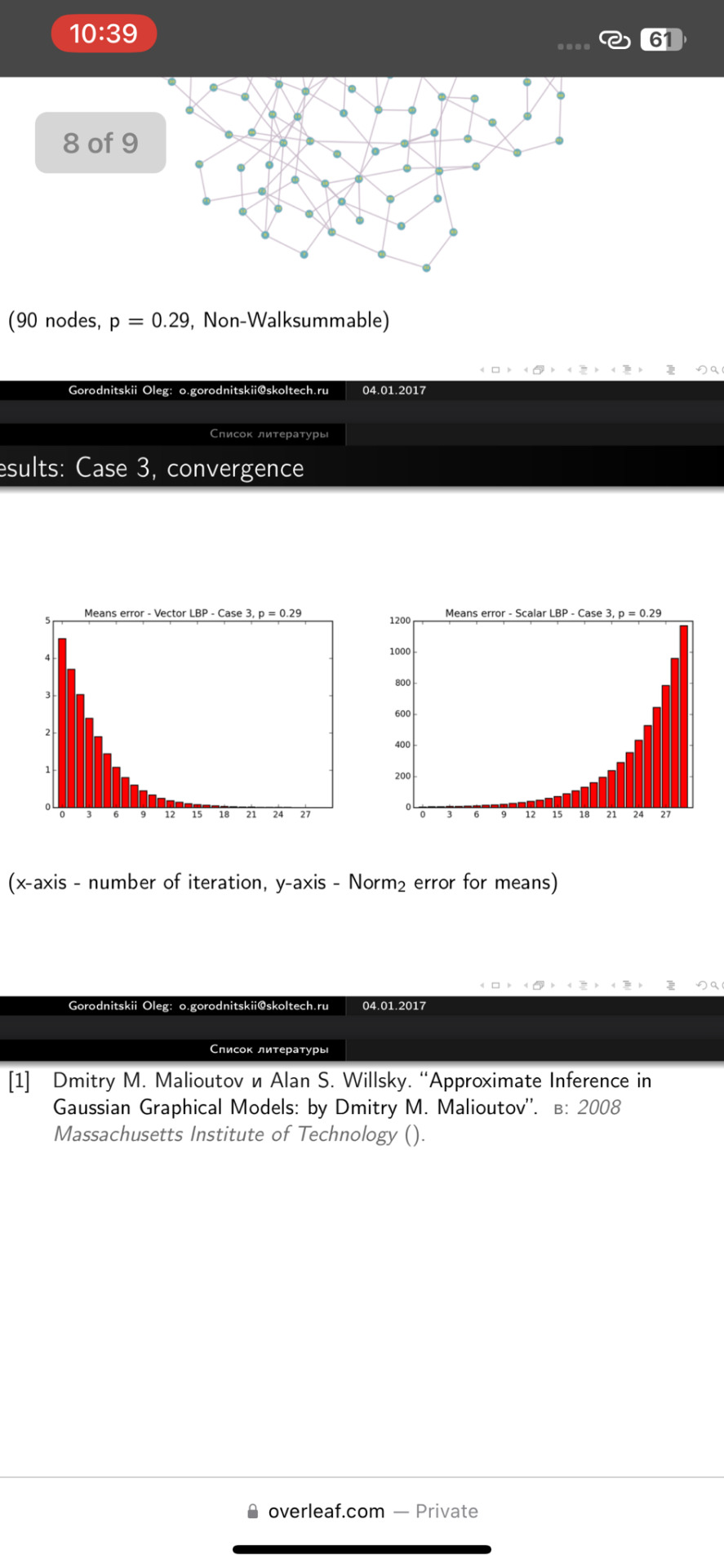
\begin{frame}{Results: Case 3}
\begin{center}
\includegraphics[scale = 0.35]{graph_3}
\end{center} (90 nodes, p = 0.29, Non-Walksummable)\\
\end{frame}
%-----------------------------------------------------------------------------------------------------
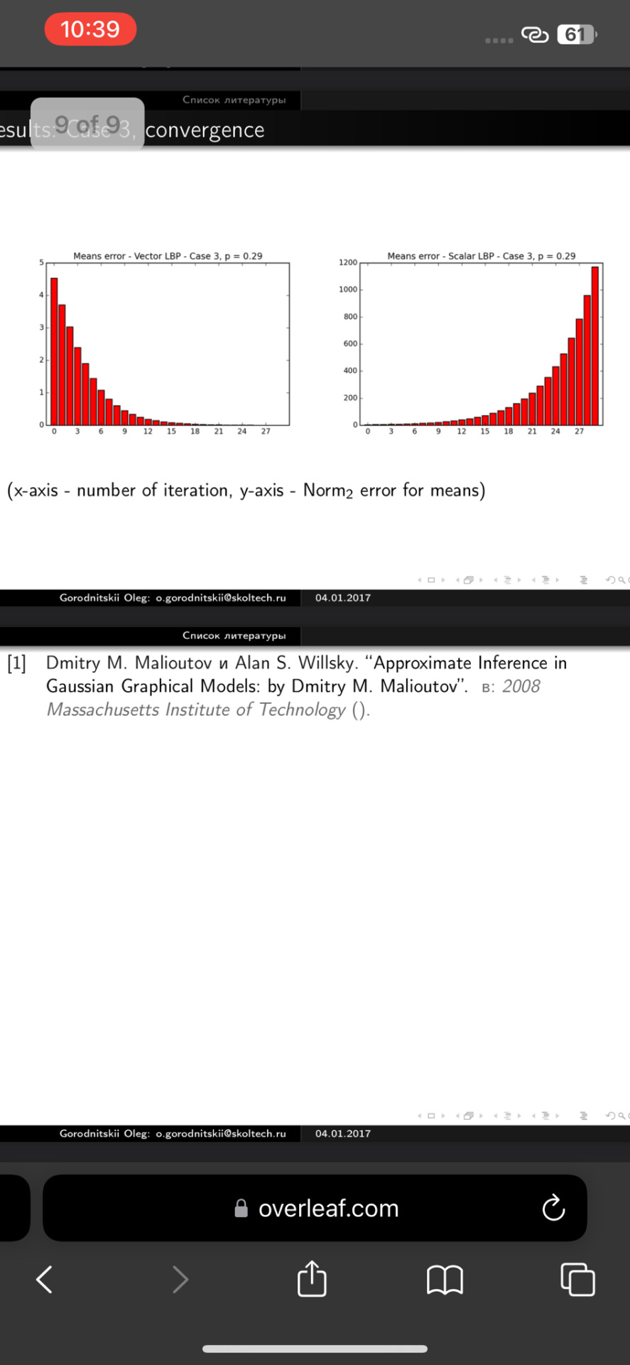
\begin{frame}{Results: Case 3, convergence}
\begin{center}
\includegraphics[scale = 0.42]{Means_err_vec_3}
\includegraphics[scale = 0.42]{Means_err_scalar_3}
\end{center} (x-axis - number of iteration, y-axis - $\text{Norm}_2$ error for means)\\
\end{frame}
\printbibliography
\end{document}
[ @taylorswift ]* 💜💜♾️♾️
0 notes
Photo

It’s that time of year again San Francisco families when we come to forest on the weekend to greet new and perspective students. Please come out to one of our open house events to meet our staff. There will be music and an art activity as well. Please RSVP first, at wildrootssf@gmail.com
#SFForestschool#Forestpreschool#SFkids#SFfamilies#wildroootssf
1 note
·
View note
Text
Reminder of blogs!
This is a side Blog for this account! While NSFW it is non-explicit.
@corabryn-blog is the primary for this account! It is very NSFW and very sexually explicit!
@sfwbabygirlcora is 100% SFW and SFFamily. Few words, mostly cute or aesthetic stuff that is not sexual. I don’t mention either this or the explicit Blog there at all in order to keep it that way!
1 note
·
View note
Photo

Last night was epic, to say the least. Congrats to Mr. and Mrs. Annear! Love you both so, so much. ❤️🍖 #anneartoeternity #hentzforthannear #sffamily http://ift.tt/2yHk8zK
0 notes
Photo

#sfmeeting #sffamily (at Bangkok, Thailand) https://www.instagram.com/p/ClJLVqVh0XY/?igshid=NGJjMDIxMWI=
0 notes
Photo

Stay tuned: We’ll tell you all about our new #cardgame tomorrow Fogust 1st 🌁 . . . #sanfrancisco #sflandmarks #haightashbury #castro #chinatown #unionsquare #lombardstreet #goldengatebridge #SF #🌁 #wip #preview #sftravel #sfsightseeing #sffog #sfsummer #sfmom #sffamily #sanfranciscobay #sanfranciscoart #fog #karlthefog #fogaholics #foglife #fogust #onlyinsf #digitalpainting #kickstarter #photoshop #illustration #kidsgames #familygame #unplugandplay #sffun #jogojoy #sfetsy (at San Francisco, California) https://www.instagram.com/p/Bl6UaejFZRw/?utm_source=ig_tumblr_share&igshid=15icmygi4v9fu
#sfsummer#kidsgames#sffog#sf#sffamily#cardgame#sfetsy#sffun#unplugandplay#kickstarter#sftravel#haightashbury#foglife#illustration#jogojoy#familygame#photoshop#chinatown#castro#sfmom#digitalpainting#preview#🌁#goldengatebridge#fogaholics#wip#sanfranciscobay#lombardstreet#sanfrancisco#karlthefog
0 notes
Text
\documentclass{beamer}
\usepackage[utf8]{inputenc}
\usepackage[english, russian]{babel} % Russian layout
\usepackage{amsmath,mathrsfs,amsfonts,amssymb}
\usepackage[demo]{graphicx}
\usepackage{subfig}
\usepackage{floatflt}
\usepackage{epic,ecltree}
\usepackage{mathtext}
\usepackage{fancybox}
\usepackage{multirow}
\usepackage{fancyhdr}
\usepackage{enumerate}
\usepackage{epstopdf}
\usepackage{amsmath}
\usepackage{blindtext}
\usepackage{scrextend}
\usepackage{mathtools}
\usepackage[T1]{fontenc}
\usepackage{textcomp}
\usepackage{siunitx}
\usepackage[noend]{algorithmic}
\usepackage{graphicx}
\usepackage{cleveref}
\usepackage{hyperref}
\usepackage{amsmath}
\usepackage{lineno}
\usepackage{caption}
\usepackage{subcaption}
\newcommand\spaceoverxrightarrow[2][\stackgap]{%
\ensurestackMath{\stackon[#1]{\xrightarrow[\phantom{#2}]{}}%
{\scriptscriptstyle #2}}}
\geometry{paperwidth=140mm,paperheight=105mm}
%\usepackage{bibentry} %for nonbibliography
\usepackage{comment}
\usepackage{color}
\usepackage{caption}
\captionsetup[figure]{labelformat=empty}
\captionsetup[table]{labelformat=empty}
\renewcommand{\thesubfigure}{\asbuk{subfigure}}
\newcommand{\X}{{\mathbf{X}}}
\newcommand{\w}{{\mathbf{w}}}
\newcommand{\A}{{\mathbf{A}}}
\newcommand{\xx}{{\mathbf{x}}}
\newcommand{\y}{{\mathbf{y}}}
\newcommand{\Hm}{{\mathbf{H}}}
\newcommand{\Wj}{\mathbf{W}_j}
\newcommand{\x}{\mathbf{x}}
\newcommand{\bx}{\mathbf{x}}
\newcommand{\bw}{\mathbf{w}}
\newcommand{\by}{\mathbf{y}}
\newcommand{\bb}{\mathbf{b}}
\newcommand{\bnu}{\mathbf{\nu}}
\newcommand{\bX}{\mathbf{X}}
\newcommand{\bY}{\mathbf{Y}}
\newcommand{\bA}{\mathbf{A}}
\newcommand{\bU}{\mathbf{U}}
\newcommand{\bV}{\mathbf{V}}
\newcommand{\bS}{\mathbf{S}}
\newcommand{\bQ}{\mathbf{Q}}
\newcommand{\bI}{\mathbf{I}}
\newcommand{\bbR}{\mathbb{R}}
\newcommand{\bchi}{\boldsymbol{\chi}}
\newcommand{\calC}{\mathcal{C}}
\newcommand{\caligc}{\mathcal{c}}
\newcommand{\calP}{\mathcal{P}}
\newcommand{\calR}{\mathcal{R}}
\newcommand{\calJ}{\mathcal{J}}
\newcommand{\calI}{\mathcal{I}}
\newcommand{\calA}{\mathcal{A}}
\newcommand{\calL}{\mathcal{L}}
\newcommand{\frakD}{\mathfrak{D}}
\newcommand{\frakM}{\mathfrak{M}}
\newcommand{\frakL}{\mathfrak{L}}
\newcommand{\frakC}{\mathfrak{C}}
\newcommand{\frakm}{\mathfrak{m}}
\newcommand{\vif}{\mathrm{VIF}}
\newcommand{\rss}{\mathrm{RSS}}
\newcommand{\tss}{\mathrm{TSS}}
\newcommand{\bic}{\mathrm{BIC}}
\newcommand{\radj}{R_{\text{adj}}^2}
\newcommand{\inter}{\text{int}}
\newcommand{\exter}{\text{ext}}
\newcommand{\T}{{\text{\tiny\sffamily\upshape\mdseries T}}}
\newcommand{\argmin}{\mathop{\arg \min}\limits}
\newcommand{\argmax}{\mathop{\arg \max}\limits}
\usetheme{Warsaw}%{Singapore}%{Warsaw}%{Warsaw}%{Darmstadt}
\usecolortheme{sidebartab}
\setbeamercolor{structure}{fg=white!10!black}
\bibliographystyle{apalike} \setbeamertemplate{bibliography item}[text]
\date{}
\title{02.24.2017}
%----------------------------------------------------------------------------------------------------------
\begin{document}
%-----------------------------------------------------------------------------------------------------
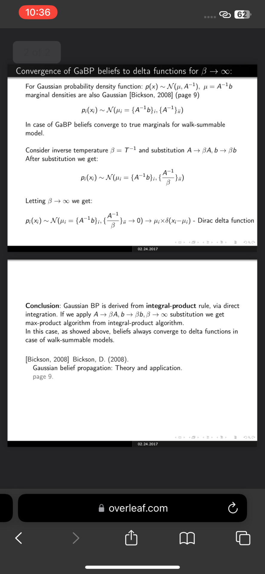
\begin{frame}{Convergence of GaBP beliefs to delta functions for $\beta \rightarrow \infty$:}
For Gaussian probability density function: $p(x) \sim \mathcal{N}(\mu, A^{-1}), \ \mu = A^{-1}b$ marginal densities are also Gaussian \cite{bic} (page 9) $$p_i(x_i) \sim \mathcal{N}(\mu_i = \{A^{-1}b\}_i,\{A^{-1}\}_{ii})$$
In case of GaBP beliefs converge to true marginals for walk-summable model.\\
Consider inverse temperature $\beta = T^{-1}$ and substitution $A \rightarrow \beta A, b \rightarrow \beta b$
After substitution we get:
$$p_i(x_i) \sim \mathcal{N}(\mu_i = \{A^{-1}b\}_i,\{\frac{A^{-1}}{\beta}\}_{ii})$$\\
Letting $\beta \rightarrow \infty$ we get:\\
$$p_i(x_i) \sim \mathcal{N}(\mu_i = \{A^{-1}b\}_i,\{\frac{A^{-1}}{\beta}\}_{ii} \rightarrow 0) \rightarrow \mu_i \times \delta(x_i - \mu_i) \text{ - Dirac delta function}$$\\
\end{frame}
%-----------------------------------------------------------------------------------------------------
\begin{frame}{}
\textbf{Conclusion}: Gaussian BP is derived from \textbf{integral-product} rule, via direct integration. If we apply $A \rightarrow \beta A, b \rightarrow \beta b, \beta \rightarrow \infty$ substitution we get max-product algorithm from integral-product algorithm.\\
In this case, as showed above, beliefs always converge to delta functions in case of walk-summable models.\\
\bibliographystyle{plain}
\bibliography{references}
\end{frame}
%-----------------------------------------------------------------------------------------------------
[ @taylorswift ]* 💜💜♾️♾️
\end{document}
0 notes
Photo

#sffamily (em AT&T Park) https://www.instagram.com/p/BnnDWDmlI8f/?utm_source=ig_tumblr_share&igshid=e5p61r6b27uq
0 notes
Text


\documentclass{beamer}
\usepackage[utf8]{inputenc}
\usepackage[english, russian]{babel} % Russian layout
\usepackage{amsmath,mathrsfs,amsfonts,amssymb}
\usepackage[demo]{graphicx}
\usepackage{subfig}
\usepackage{floatflt}
\usepackage{epic,ecltree}
\usepackage{mathtext}
\usepackage{fancybox}
\usepackage{multirow}
\usepackage{fancyhdr}
\usepackage{enumerate}
\usepackage{epstopdf}
\usepackage{amsmath}
\usepackage{blindtext}
\usepackage{scrextend}
\usepackage{mathtools}
\usepackage[T1]{fontenc}
\usepackage{textcomp}
\usepackage{siunitx}
\usepackage[noend]{algorithmic}
\usepackage{graphicx}
\usepackage{cleveref}
\usepackage{hyperref}
\usepackage{amsmath}
\usepackage{lineno}
\usepackage{caption}
\usepackage{subcaption}
\geometry{paperwidth=140mm,paperheight=105mm}
%\usepackage{bibentry} %for nonbibliography
\usepackage{comment}
\usepackage{color}
\usepackage{caption}
\captionsetup[figure]{labelformat=empty}
\captionsetup[table]{labelformat=empty}
\renewcommand{\thesubfigure}{\asbuk{subfigure}}
\newcommand{\X}{{\mathbf{X}}}
\newcommand{\w}{{\mathbf{w}}}
\newcommand{\A}{{\mathbf{A}}}
\newcommand{\xx}{{\mathbf{x}}}
\newcommand{\y}{{\mathbf{y}}}
\newcommand{\Hm}{{\mathbf{H}}}
\newcommand{\Wj}{\mathbf{W}_j}
\newcommand{\x}{\mathbf{x}}
\newcommand{\bx}{\mathbf{x}}
\newcommand{\bw}{\mathbf{w}}
\newcommand{\by}{\mathbf{y}}
\newcommand{\bb}{\mathbf{b}}
\newcommand{\bnu}{\mathbf{\nu}}
\newcommand{\bX}{\mathbf{X}}
\newcommand{\bY}{\mathbf{Y}}
\newcommand{\bA}{\mathbf{A}}
\newcommand{\bU}{\mathbf{U}}
\newcommand{\bV}{\mathbf{V}}
\newcommand{\bS}{\mathbf{S}}
\newcommand{\bQ}{\mathbf{Q}}
\newcommand{\bI}{\mathbf{I}}
\newcommand{\bbR}{\mathbb{R}}
\newcommand{\bchi}{\boldsymbol{\chi}}
\newcommand{\calC}{\mathcal{C}}
\newcommand{\caligc}{\mathcal{c}}
\newcommand{\calP}{\mathcal{P}}
\newcommand{\calR}{\mathcal{R}}
\newcommand{\calJ}{\mathcal{J}}
\newcommand{\calI}{\mathcal{I}}
\newcommand{\calA}{\mathcal{A}}
\newcommand{\calL}{\mathcal{L}}
\newcommand{\frakD}{\mathfrak{D}}
\newcommand{\frakM}{\mathfrak{M}}
\newcommand{\frakL}{\mathfrak{L}}
\newcommand{\frakC}{\mathfrak{C}}
\newcommand{\frakm}{\mathfrak{m}}
\newcommand{\vif}{\mathrm{VIF}}
\newcommand{\rss}{\mathrm{RSS}}
\newcommand{\tss}{\mathrm{TSS}}
\newcommand{\bic}{\mathrm{BIC}}
\newcommand{\radj}{R_{\text{adj}}^2}
\newcommand{\inter}{\text{int}}
\newcommand{\exter}{\text{ext}}
\newcommand{\T}{{\text{\tiny\sffamily\upshape\mdseries T}}}
\newcommand{\argmin}{\mathop{\arg \min}\limits}
\newcommand{\argmax}{\mathop{\arg \max}\limits}
\usetheme{Warsaw}%{Singapore}%{Warsaw}%{Warsaw}%{Darmstadt}
\usecolortheme{sidebartab}
\setbeamercolor{structure}{fg=white!10!black}
\bibliographystyle{apalike} \setbeamertemplate{bibliography item}[text]
\date{}
\title{02.17.2017}
% A subtitle is optional and this may be deleted
\subtitle{GaBP preconditioned conjugate gradients method}
\author{Gorodnitskii Oleg: o.gorodnitskii@skoltech.ru}
\AtBeginSubsection[GaBP preconditioned conjugate gradient method]
{
\begin{frame}<beamer>{Outline}
\tableofcontents[currentsection,currentsubsection]
\end{frame}
}
%----------------------------------------------------------------------------------------------------------
\begin{document}
\begin{frame}
\titlepage
\end{frame}
%-----------------------------------------------------------------------------------------------------
\begin{frame}{Bickson-Dolev scheme (I):}
Consider linear system $Ax = b$, $A \in \text{SPD}(R^{n \times n}), A \not\in \text{SDD}(R^{n \times n})$\\
Assume A is normalized and admits representation: $A = I - R$\\
Task: to obtain $\widetilde{x}$ such that ||$\widetilde{x} - x^{*}$|| < $\varepsilon$, where $x^{*} = A^{-1}b$\\
General concept: two cycles - inner and outer, inner embedded into the outer.\\
Basic (Bickson's) scheme: outer cycle = Fixed-point iteration, inner cycle = GaBP.\\
Fixed-point iterative scheme:
$$x^{(t+1)} = \frac{b + \Gamma x^{(t)}}{A + \Gamma}$$
where $\Gamma$ such that: $(A + \Gamma) \in \text{SDD}$.\\
In Base case: $\Gamma = wI, I - \text{identity matrix}$, $w > w_0 = \rho(|R|) - 1$\\
( $w_0$ - threshold for $w$ (minimal w) such that $(A + \widetilde{w}I) \in \text{SDD}(R^{n \times n}), \forall \widetilde{w} > w_0$ and $(A + \widetilde{w}I) \notin \text{SDD}(R^{n \times n}), \forall \widetilde{w} \leq w_0$)
\end{frame}
%-----------------------------------------------------------------------------------------------------
\begin{frame}{Bickson-Dolev scheme (II):}
Function GaBP($\widetilde{A}, b$) returns $\widetilde{A}^{-1}b$ for walk-summable $\widetilde{A}$, calculating it via Gaussian BP.\\
Whole process of solution $Ax = b, A \notin \text{SDD}, A = I - R$ by steps:\\
\begin{itemize}
\item w = $k \times (\rho(|R|) - 1), k > 1.0$
\item $x^{(0)} = $ GaBP($A + wI, b$)
\item Iterate:
\begin{itemize}
\item $b^{(t+1)} = b + wI*x^{(t)}$
\item $x^{(t+1)} = $ GaBP($A + wI, b^{(t+1)}$)
\item If $||x^{(t+1)} - x^{(t)}|| < \varepsilon$ then exit.
\end{itemize}
\item Solution $\widetilde{x}$ = $x^{(t+1)}$
\end{itemize}\\
Fixed-point iteration interpretation:\\
$x^{(t+1)} = \frac{b + wI x^{(t)}}{A + wI}$ can be rewritten in a form:\\
$x^{(t+1)} = Tx^{(t)} + \psi_{k}$ - Fixed-point iterations scheme with $T = \frac{wI}{A + wI}, \psi_{k} = \frac{b}{A + wI}$.
\end{frame}
%-----------------------------------------------------------------------------------------------------
\begin{frame}{Bickson-Dolev scheme (III):}
Definitions:\\
m = $\lambda_{min}(A)$\\
M = $\lambda_{max}(A)$\\
w - parameter, defined as above\\
$\varepsilon$ - demanded precisions of answer (outer cycle precision by argument)\\
For Fixed-point iteration scheme of form $x^{(t+1)} = Tx^{(t)} + \psi_{k}$, where $T$ is a linear operator, convergence rate is determined by $\rho(T)$ - spectral radius of $T$.\\
For precision $\varepsilon$ (by argument) number of iteration is $k \approx \frac{log(\varepsilon)}{log(\rho(T))}$ (see page 226 of <<Lebedev - Functional analysis and computational mathematics>>).\\
For Bickson's scheme $T = \frac{wI}{A + wI}$ and number of outer cycle iterations:\\
$$k \approx \frac{log(\epsilon)} {log(\frac{w}{w + m})}$$
\textbf{Idea:} replacing Fixed-point iteration with Chebyshev iteration (or Preconditioned conjugate gradient method) can significantly reduce the number of outer cycle iterations.
\end{frame}
%-----------------------------------------------------------------------------------------------------
\begin{frame}{Preconditioned conjugate gradient method}
\noindent\begin{minipage}{0.6\textwidth}% adapt widths of minipages to your needs
\includegraphics[width=\linewidth]{CG_prec}
\end{minipage}%
\hfill%
\begin{minipage}{0.4\textwidth}\raggedleft
\includegraphics[width=\linewidth]{prec}\\
The aim of algorithm is to solve $Ax = b$, with fixed precision ||$\widetilde{x} - x^{*}$|| < $\varepsilon$\bigskip
As a preconditioner we can use GaBP(M, $r_{k+1}$) with $M = A + \Gamma$, where $\Gamma$ satisfies $(A + \Gamma) \in \text{SDD}$.\bigskip
Then step $z_{k+1} := M^{-1}r_{k+1}$ is replaced with $z_{k+1} := GaBP(A + \Gamma, r_{k+1})$
\bigskip
\end{minipage}
\end{frame}
%-----------------------------------------------------------------------------------------------------
\begin{frame}{Results:}
Final scheme: preconditioned conjugate gradient method with GaBP as a preconditioner.\\
This approach allows to significantly reduce number of outter cycle iterations in comparsion with Base scheme (Fixed-point iterations in outer cycle)\\
Let Base(k) to be the number of outer cycle iterations in case of Basic scheme and CGBP(k) - in case of CG + GaBP scheme.\\
Comparison of number of outer cycle iterations for different arbitrary SPD matrices $A \in R^{n \times n}$:
\begin{itemize}
\item Case 1: n = 50: Base(k) = 1457, CGBP(k) = 30\\
\item Case 2: n = 100, Base(k) = 2281, CGBP(k) = 35\\
\item Case 3: n = 500, Base(k) = 4855, CGBP(k) = 44\\
\item Case 4: n = 1000, Base(k) = 5642, CGBP(k) = 51
\end{itemize}
\end{frame}
%-----------------------------------------------------------------------------------------------------
\end{document}
0 notes