#pvalue
Explore tagged Tumblr posts
Visit Tumblr Blog
Explore Tumblr blogs with no restrictions, modern design and the best experience.
Last Seen Tumblr Blogs


Fun Fact
The “We are the 99%” Tumblr blog became the slogan for the Occupy Wall Street movement.
Text

Statistical Significance
Statistical significance is a key concept in research and data analysis, representing the likelihood that a result or relationship observed in a study is not due to random chance. In hypothesis testing, a result is considered statistically significant if the p-value falls below a pre-determined threshold (commonly 0.05), indicating strong evidence against the null hypothesis. This concept helps researchers determine the validity of their findings and ensure that conclusions drawn from data have a low probability of being due to random variation.
Website : sciencefather.com
Nomination: Nominate Now
Registration: Register Now
Contact Us: [email protected]
#sciencefather#researcher#Professor#Lecturer#Scientist#Scholar#BestTeacherAward#BestPaperAward#StatisticalSignificance#PValue#HypothesisTesting#DataAnalysis#StatisticalAnalysis#SignificanceLevel#NullHypothesis#ConfidenceIntervals#ResearchMethods#ScientificResearch
0 notes
Text
p-Value (Statistics made simple)
What is the p-Value in statistics? The p-value is one of the most important quantities in statistics for interpreting hypothesis tests. source
0 notes
Text
Chi-Square Test of independence between mars crater depth and number of layers
We prepare the environment as usual
import pandas as pd import scipy.stats import matplotlib.pyplot as plt Read the file data = pd.read_csv('marscrater_pds.csv', delimiter=",")
The Mars Crater Dataset does not provide two categorical variables, so in order to perform some Chi-Square Tests, we need to categorize one variable. Following the previous exercise, I choose depth for this assignment.
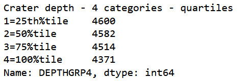
#4 Categories split (use qcut function & ask for 4 groups) print ('Crater depth - 4 categories - quartiles') sub1['DEPTHGRP4']=pd.qcut(sub1.DEPTH_RIMFLOOR_TOPOG, 4, labels=["1=25th%tile","2=50%tile","3=75%tile","4=100%tile"]) c4 = sub1['DEPTHGRP4'].value_counts(sort=False, dropna=True) print(c4)
#contingency table of observed counts ct1=pd.crosstab(sub1['DEPTHGRP4'], sub1['NUMBER_LAYERS']) print (ct1) #column percentages colsum=ct1.sum(axis=0) colpct=ct1/colsum print(colpct)
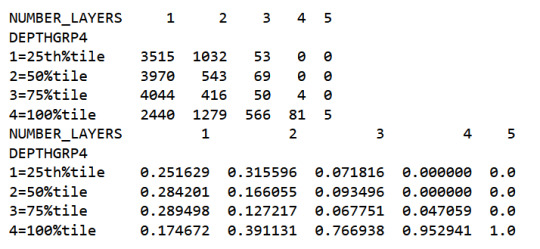
All craters with 5 layers are in the 100% quartile.
#chi-square print ('chi-square value, p value, expected counts') cs1= scipy.stats.chi2_contingency(ct1) print (cs1)
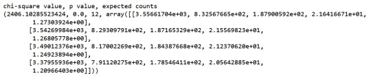
The high chi-square and low p value show that at least two groups are not independent from each other.
Post hoc comparisons
We can iterate through all combinations to find groups where the null hypothesis can be rejected. I use nested for loops to go through all 10 comparisons.
pvalues = {} numcomp = 0 sub2 = sub1.copy() for i in range(1,6): for j in range(i + 1, 6): recode = {} recode[i] = i recode[j] = j #print() compstr = 'COMP'+str(j)+'v'+str(i) sub2[compstr]= sub1['NUMBER_LAYERS'].map(recode) # contingency table of observed counts ct=pd.crosstab(sub2['DEPTHGRP4'], sub2[compstr]) #print (ct) # column percentages colsum=ct.sum(axis=0) colpct=ct/colsum #print(colpct) print ('chi-square value, p value, expected counts') cs= scipy.stats.chi2_contingency(ct) #print (cs) pvalues[compstr]= cs[1] numcomp = numcomp + 1 bonferroni = 0.05/numcomp print (pvalues) print('Bonferroni adjusted p: '+ str(bonferroni)) print ({l:(p < bonferroni) for l,p in pvalues.items()})
The commented out print statements can be uncommented to see the result of each comparison. Important for this study is the collection in pvalues. The Bonferroni adjusted p is calculated based on the number of combinations calculated.
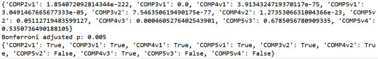
The post hoc comparisons show that mean depth is indeed dependent of the number of layers, if they are between 1 and 4. 5 layered craters have independent mean depths in comparison with 1 and 2 layered craters only. So there is no significant mean depth difference between 5 layered craters and craters with 3 or 4 layers.
0 notes
Text
'''' Autor: Renato Ferreira da Silva Projeto: Monitoramento dos Zeros da Função Zeta de Riemann Descrição: Este código analisa estatisticamente os espaçamentos entre os zeros não triviais da função zeta de Riemann, utilizando técnicas de aprendizado de máquina e detecção de desvios estatísticos. """
import numpy as np import mpmath import matplotlib.pyplot as plt from scipy.stats import ks_2samp, gamma from sklearn.preprocessing import RobustScaler from tqdm import tqdm import pandas as pd
Configurações globais
N_ZEROS_BASELINE = 20000 # Número de zeros iniciais para baseline WINDOW_SIZE = 100 # Tamanho da janela de análise SIM_ITERATIONS = 150 # Número de iterações de simulação
class RiemannMonitor: def init(self): self.baseline = None self.gue_reference = None self.scaler = RobustScaler() self._initialize_system()def _initialize_system(self): """Carrega os zeros iniciais e cria a baseline""" print("⏳ Calculando zeros base...") self.zeros_baseline = self._fetch_zeros(1, N_ZEROS_BASELINE) self._process_baseline() def _fetch_zeros(self, start, end): """Obtém zeros da função zeta com mpmath""" return [float(mpmath.zetazero(n).imag) for n in tqdm(range(start, end+1))] def _process_baseline(self): """Processa os espaçamentos normalizados""" spacings = np.diff(self.zeros_baseline) self.mean_spacing = np.mean(spacings) self.baseline = spacings / self.mean_spacing self.gue_reference = np.random.gamma(1, 1, len(self.baseline)) def analyze_new_zeros(self, new_zeros): """Analisa um novo conjunto de zeros""" new_spacings = np.diff(new_zeros) / self.mean_spacing return self._analyze_spacings(new_spacings) def _analyze_spacings(self, spacings): """Executa análise completa dos espaçamentos""" # Análise estatística stats = { 'ks_baseline': ks_2samp(self.baseline, spacings), 'ks_gue': ks_2samp(self.gue_reference, spacings), 'moments': { 'mean': np.mean(spacings), 'std': np.std(spacings), 'skew': gamma.fit(spacings)[0] } } return stats def run_simulation(self): """Executa simulação controlada com dados sintéticos""" results = [] for i in tqdm(range(SIM_ITERATIONS), desc="🚀 Simulando cenários"): # Gera dados sintéticos com desvios programados if i % 10 == 0: data = np.random.gamma(1, 1.15, WINDOW_SIZE) # Desvio de média elif i % 7 == 0: data = np.random.weibull(1.2, WINDOW_SIZE) # Desvio distribucional else: data = np.random.gamma(1, 1, WINDOW_SIZE) # Dados normais # Analisa e armazena resultados analysis = self._analyze_spacings(data) results.append({ 'batch': i, 'mean': np.mean(data), 'p_value_baseline': analysis['ks_baseline'].pvalue, 'p_value_gue': analysis['ks_gue'].pvalue }) return pd.DataFrame(results)
Executar o código
if name == "main": monitor = RiemannMonitor() new_zeros = monitor._fetch_zeros(N_ZEROS_BASELINE+1, N_ZEROS_BASELINE+WINDOW_SIZE) analysis = monitor.analyze_new_zeros(new_zeros)# Exibir resultados da simulação df_results = monitor.run_simulation() print("Resultados da Simulação:") print(df_results.head())
0 notes
Text
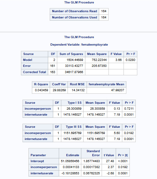
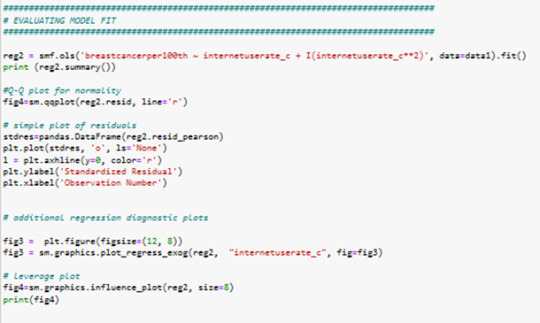
Test a Multiple Regression Model
We will be using the Gapminder dataset to study the relation between response variable femaleemployrate and explanatory variables incomeperperson and internetuserate.
Code
Libname data '/home/u47394085/Data Analysis and Interpretation';
Proc Import Datafile='/home/u47394085/Data Analysis and Interpretation/gapminder.csv' Out=data.Gapminder Dbms=csv replace; Run;
Proc Means Data=data.Gapminder NMISS; Run;
Data Gapminder_Linear_Model; Set data.Gapminder; If femaleemployrate=. OR internetuserate=. OR incomeperperson=. Then Delete; Run;
Proc Means Data=Gapminder_Linear_Model NMISS; Run;
Title 'Mean of the Explanatory Variable'; Proc Means Data=Gapminder_Linear_Model Mean; Var incomeperperson; Run; Title;
Proc Glm Data=Gapminder_Linear_Model Plots=All; Model femaleemployrate = incomeperperson internetuserate; Run; Quit;
Output:
Interpretation
The linear regression equation that we have received is as below:
femaleemployrate=51.05856456+0.00041133×incomeperperson + (-0.18128653)xinternetuserate
We say, if the incomeperson for a country is $ 8000 and internetuserate is 35 then it's estimated femaleemployrate would be:
femaleemployrate =21.351071+0.00168031×8000 + (-0.18128653)x35
femaleemployrate = 48
Meaning the country having around $ 8000 as it's per capita income and with 35 internet users per 100 of it's population would have around 48 per 100 females (age>15) employed that year.
Incomeperperson has a positive correlation whereas internetuserate has a negative correlation with femaleemployrate.
The p values for both the explanatory variables indicate that both are significant.
One interesting thing to note is that, both these explanatory variables are insignificant when evaluated for significance against the response variable as their individual pvalues are > 0.05.
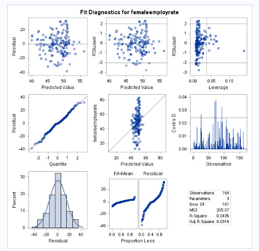
Please find below the interpretation of the various plots:
QQ Plot - The data may not be normally distributed
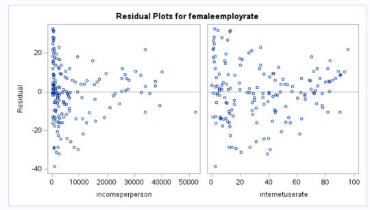
Residual Plot - The variance may not be constant
Leverage Plot - There may be some influential observations.
0 notes
Text
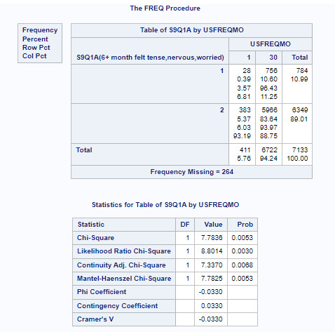
Anxiety and Smoking
This is an exemple comparing USFREQMO as 1 and 30. Within those two distant frequency, we got a high p value, compared with the pvalue adjusted, that should be less than 0.003. So it's clear that we don't have associating between frequency of smoking and felt tense, nervous or worried for a period of 6 months or more.
the code:
/* Definindo a biblioteca de dados */ LIBNAME mydata "/courses/d1406ae5ba27fe300" access=readonly;
/* Criando um novo conjunto de dados */ DATA new; set mydata.nesarc_pds;/* Definindo rótulos para variáveis */ LABEL TAB12MDX = "Tobacco Dependence Past 12 Months" CHECK321 = "Smoked Cigarettes in Past 12 Months" S3AQ3B1 = "Usual Smoking Frequency" S3AQ3C1 = "Usual Smoking Quantity" S9Q1A = "6+ month felt tense,nervous,worried"; /* Tratamento de dados ausentes */ IF S3AQ3B1 = 9 THEN S3AQ3B1 = .; IF S3AQ3C1 = 99 THEN S3AQ3C1 = .; IF S9Q1A = 9 THEN S9Q1A = .; /* Mapeamento da frequência de fumo para categorias */ IF S3AQ3B1 = 1 THEN USFREQMO = 30; ELSE IF S3AQ3B1 = 2 THEN USFREQMO = 22; ELSE IF S3AQ3B1 = 3 THEN USFREQMO = 14; ELSE IF S3AQ3B1 = 4 THEN USFREQMO = 5; ELSE IF S3AQ3B1 = 5 THEN USFREQMO = 2.5; ELSE IF S3AQ3B1 = 6 THEN USFREQMO = 1; /* Calculando o número estimado de cigarros por mês */ NUMCIGMO_EST = USFREQMO * S3AQ3C1; /* Calculando pacotes por mês e categorizando */ PACKSPERMONTH = NUMCIGMO_EST / 20; IF PACKSPERMONTH LE 5 THEN PACKCATEGORY = 3; ELSE IF PACKSPERMONTH LE 10 THEN PACKCATEGORY = 7; ELSE IF PACKSPERMONTH LE 20 THEN PACKCATEGORY = 15; ELSE IF PACKSPERMONTH LE 30 THEN PACKCATEGORY = 25; ELSE IF PACKSPERMONTH GT 30 THEN PACKCATEGORY = 58; /* Subconjunto de dados para incluir apenas fumantes dos últimos 12 meses entre 18-60 anos */ IF CHECK321 = 1; IF AGE GT 18; IF AGE LE 60; /*IF USFREQMO = 1 OR USFREQMO = 2.5; IF USFREQMO = 1 OR USFREQMO = 5; IF USFREQMO = 1 OR USFREQMO = 14; IF USFREQMO = 1 OR USFREQMO = 22;*/ IF USFREQMO = 1 OR USFREQMO = 30; /*IF USFREQMO = 2.5 OR USFREQMO = 5; IF USFREQMO = 2.5 OR USFREQMO = 14; IF USFREQMO = 2.5 OR USFREQMO = 22; IF USFREQMO = 2.5 OR USFREQMO = 30; IF USFREQMO = 5 OR USFREQMO = 14; IF USFREQMO = 5 OR USFREQMO = 22; IF USFREQMO = 5 OR USFREQMO = 30; IF USFREQMO = 14 OR USFREQMO = 22; IF USFREQMO = 14 OR USFREQMO = 30; IF USFREQMO = 22 OR USFREQMO = 30;*/ /* Ordenando os dados por IDNUM */ PROC SORT; BY IDNUM; PROC FREQ; TABLES S9Q1A*USFREQMO/CHISQ;
RUN;
0 notes
Text
Panel VAR in Stata and PVAR-DY-FFT
Preparation
xtset pros mm (province, month)
Endogenous variables:
global Y loan_midyoy y1 stock_pro
Provincial medium-term loans year-on-year (%)
Provincial 1-year interest rate (%) (NSS model estimate, not included in this article) (%)
provincial stock return
Exogenous variables:
global X lnewcasenet m2yoy reserve_diff
Logarithm of number of confirmed cases
M2 year-on-year
reserve ratio difference
Descriptive statistics:
global V loan_midyoy y1 y10 lnewcasenet m2yoy reserve_diff sum2docx $V using "D.docx", replace stats(N mean sd min p25 median p75 max ) title("Descriptive statistics")
VarName Obs Mean SD Min P25 Median P75 Max
loan_midyoy 2232 13.461 7.463 -79.300 9.400 13.400 16.800 107.400
y1 2232 2.842 0.447 1.564 2.496 2.835 3.124 4.462
stock_pro 2232 0.109 6.753 -24.485 -3.986 -0.122 3.541 73.985
lnewcasenet 2232 1.793 2.603 0.000 0.000 0.000 3.434 13.226
m2yoy 2232 0.095 0.012 0.080 0.085 0.091 0.105 0.124
reserve_diff 2232 -0.083 0.232 -1.000 0.000 0.000 0.000 0.000
Check for unit root:
foreach x of global V { xtunitroot ips `x',trend }
Lag order
pvarsoc $Y , pinstl(1/5)
pvaro(instl(4/8)): Specifies to use the fourth through eighth lags of each variable as instrumental variables. In this case, in order to deal with endogeneity issues, relatively distant lags are chosen as instrumental variables. This means that when estimating the model, the current value of each variable is not directly affected by its own recent lagged value (first to third lag), thus reducing the possibility of endogeneity.
pinstl(1/5): Indicates using lags from the highest lag to the fifth lag as instrumental variables. Specifically, for the PVAR(1) model, the first to fifth lags are used as instrumental variables; for the PVAR(2) model, the second to sixth lags are used as instrumental variables, and so on. The purpose of this approach is to provide each model variable with a set of instrumental variables that are related to, but relatively independent of, its own lag structure, thereby helping to address endogeneity issues.
CD test (Cross-sectional Dependence Test): This is a test to detect whether there is cross-sectional dependence (ie, correlation between different individuals) in panel data. Values close to 1 generally indicate the presence of strong cross-sectional dependence. If there is cross-sectional dependence in the data, cluster-robust standard errors can be used to correct for this.
J-statistic: The J-statistic that detects model over-identification of constraints and is usually related to the effectiveness of instrumental variables.
J pvalue: The p value of the J statistic, used to determine whether the instrumental variable is valid. A low p-value (usually less than 0.05) means that at least one of the instrumental variables is probably not applicable.
MBIC, MAIC, MQIC: These are different information criterion values, used for model selection. Lower values generally indicate a better model.
MBIC: Bayesian Information Criterion.
MAIC: Akaike Information Criterion.
MQIC: Quantile information criterion.

Interpretation: The p-values of the J-test are 0.00 and 0.63 for Lag 1 and Lag 2 respectively. The p-value for the first lag is very low, indicating possible instrumental variable inefficiency. The p-value for the second lag is higher, indicating that instrumental variables may be effective. In this example, Lag 2 seems to be the optimal choice because its MBIC, AIC, and MQIC values are relatively low. However, it should be noted that the CD test shows that there is cross-sectional dependence, which may affect the accuracy of model estimation.
Model estimation:
pvar $Y, lags(2) instlags(1/4) fod exog($X) gmmopts(winitial(identity) wmatrix(robust) twostep vce(cluster pros))
pvar: This is the Stata command that calls the PVAR model.
$Y: These are the endogenous variables included in the model.
$X: These are exogenous variables included in the model.
lags(2): Specifies to include 2-period lags for each variable in the PVAR model.
number of lag periods for the variable
instlags(1/4): This is the number of lags for the specified instrumental variable. Here, it tells Stata to use the first to fourth lags as instrumental variables. This is to address possible endogeneity issues, i.e. possible interactions between variables in the model.
Lag order selection criteria:
Information criterion: Statistical criteria such as AIC and BIC can be used to judge the choice of lag period.
Diagnostic tests: Use diagnostic tests of the model (e.g. Q(b), Hansen J overidentification test) to assess the appropriateness of different lag settings.
fod/fd: medium fixed effects.
fod: The Helmert transformation is a forward mean difference method that compares each observation to the mean of its future observations. This method makes more efficient use of available information than simple difference-in-difference methods when dealing with fixed effects, especially when the time dimension of panel data is short.
A requirement of the Helmert transformation on the data is that the panel must be balanced (i.e., for each panel unit, there are observations at all time points).
fd: Use first differences to remove panel-specific fixed effects. In this method, each observation is subtracted from its observation in the previous period, thus eliminating the influence of time-invariant fixed effects. First difference is a common method for dealing with fixed effects in panel data, especially when there is a trend or horizontal shift in the data over time.
Usage Scenarios and Choices: If your panel data is balanced and you want to utilize time series information more efficiently, you may be inclined to use the Helmert transformation. First differences may be more appropriate if the data contain unbalanced panels or if there is greater concern with removing possible time trends and horizontal shifts.
exog($X): This option is used to specify exogenous variables in the model. Exogenous variables are assumed to be variables that are not affected by other variables in the model.
gmmopts(winitial(identity) wmatrix(robust) twostep vce(cluster pros))
winitial(identity): Set the initial weight matrix to the identity matrix.
wmatrix(robust): Use a robust weight matrix.
twostep: Use the two-step GMM estimation method.
vce(cluster pros): Specifies the standard error of clustering robustness, and uses `pros` as the clustering variable.
GMM criterion function
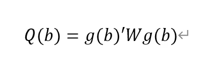
Final GMM Criterion Q(b) = 0.0162: The GMM criterion function (Q(b)) is a mathematical expression that measures how consistent your model parameter estimates (b) are with these moment conditions. Simply put, it measures the gap between model parameters and theoretical or empirical expectations.
is a vector of moment conditions. These moment conditions are a series of assumptions or constraints set based on the model. They usually come in the form of expected values (expectations) that represent the conditions that the model parameter b should satisfy.
W is a weight matrix used to assign different weights to different moment conditions.
b is a vector of model parameters. The goal of GMM estimation is to find the optimal b to minimize Q(b).
No. of obs = 2077: This means there are a total of 2077 observations in the data set.
No. of panels = 31: This means that the data set contains 31 panel units.
Ave. no. of T = 67.000: Each panel unit has an average of 67 time point observations.
Coefficient interpretation (not marginal effects)
L1.loan_midyoy: 0.8034088: When the one-period lag of loan_midyoy increases by one unit, the current period's loan_midyoy is expected to increase by approximately 0.803 units. This coefficient is statistically significant (p-value 0.000), indicating that the one-period lag has a significant positive impact on the current value.
L2.loan_midyoy: 0.1022556: When the two-period lag of loan_midyoy increases by one unit, the current period's loan_midyoy is expected to increase by approximately 0.102 units. This coefficient is not statistically significant (p-value of 0.3), indicating that the effect of the two-period lag on the current value may not be significant.

overidentification test
pvar $Y, lags(2) instlags(1/4) fod exog($X) gmmopts(winitial(identity) wmatrix(robust) twostep vce(cluster pros)) overid (written in one line)
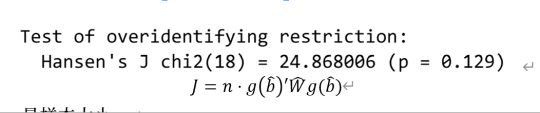
Statistics: Hansen's J chi2(18) = 24.87 means that the chi-square statistic value of the Hansen J test is 24.87 and the degrees of freedom are 18.
P-value: (p = 0.137) means that the p-value of this test is 0.129. Since the p-value is higher than commonly used significance levels (such as 0.05 or 0.01), this indicates that there is insufficient evidence to reject the null hypothesis. In the Hansen J test, the null hypothesis is that all instrumental variables are exogenous, that is, they are uncorrelated with the error term. Instrumental variables may be appropriate.
Stability check:
pvarstable

Eigenvalues: Listed eigenvalues include their real and imaginary parts. For example, 0.9271743 is a real eigenvalue. 0.0337797±0.326651i is a pair of conjugate complex eigenvalues.
Modulus: The module of an eigenvalue is its distance from the origin on the complex plane. It is calculated as the square root of the sum of the squares of the real and imaginary parts.
Stability condition: The stability condition of the PVAR model requires that the modules of all eigenvalues must be less than or equal to 1 (that is, all eigenvalues are located within the unit circle).
Granger causality:
pvargranger
Ho (null hypothesis): The excluded variable is not a Granger cause (i.e. does not have a predictive effect on the variables in the equation).
Ha (alternative hypothesis): The excluded variable is a Granger cause (i.e. has a predictive effect on the variables in the equation).

For the stock_pro equation:
loan_midyoy: chi2 = 6.224 (degrees of freedom df = 2), p-value = 0.045. There is sufficient evidence to reject the null hypothesis, indicating that loan_midyoy is the Granger cause of stock_pro.
y1: chi2 = 0.605 (degrees of freedom df = 2), p-value = 0.739. There is insufficient evidence to reject the null hypothesis indicating that y1 is not the Granger cause of stock_pro.
Margins:
The PVAR model involves the dynamic interaction of multiple endogenous variables, which means that the current value of a variable is not only affected by its own past values, but also by the past values of other variables. In this case, the margins command may not be suitable for calculating or interpreting the marginal effects of variables in the model, because these effects are not fixed but change dynamically with time and the state of the model. The following approaches may be considered:
Impulse response analysis
Impulse response analysis: In the PVAR model, the more common analysis method is to perform impulse response analysis (Impulse Response Analysis), which can help understand how the impact of one variable affects other variables in the system over time.
pvarirf,oirf mc(200) tab
Orthogonalized Impulse Response Function (OIRF): In some economic or financial models, orthogonalized processing may be more realistic, especially when analyzing policy shocks or other clearly distinguished externalities. During impact. If the shocks in the model are assumed to be independent of each other, then OIRF should be used. Orthogonalization ensures that each shock is orthogonal (statistically independent) through a mathematical process (such as Cholisky decomposition). This means that the effect of each shock is calculated controlling for the other shocks.
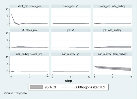
When stock_pro is subject to a positive shock of one standard deviation, loan_midyoy is expected to decrease slightly in the first period, with a specific response value of -0.0028833, indicating that loan_midyoy is expected to decrease by approximately 0.0029 units.
This effect gradually changes over time. For example, in the second period, the shock response of loan_midyoy to stock_pro is 0.0700289, which means that loan_midyoy is expected to increase by about 0.0700 units.
pvarirf, mc(200) tab
For some complex dynamic systems, non-orthogonalized IRF may be better able to capture the actual interactions between variables within the system. Non-orthogonalized impulse response function: If you do not make the assumption that the shocks are independent of each other, or if you believe that there is some inherent interdependence between the variables in the model, you may choose a non-orthogonalized IRF.
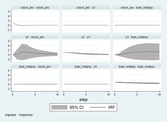
When stock_pro is impacted: In period 1, loan_midyoy has a slightly negative response to the impact on stock_pro, with a response value of -0.0004269.
This effect gradually changes over time. For example, in period 2, the response value is 0.0103697, indicating that loan_midyoy is expected to increase slightly.
Forecast error variance decomposition
Forecast Error Variance Decomposition is also a useful tool for analyzing the dynamic relationship between variables in the PVAR model.
Time point 0: The contribution of all variables is 0, because at the initial moment when the impact occurs, no variables have an impact on loan_midyoy.
Time point 1: The forecast error variance of loan_midyoy is completely explained by its own shock (100%), while the contribution of y1 and stock_pro is 0.
Subsequent time points: For example, at time point 10, about 99.45% of the forecast error variance of loan_midyoy is explained by the shock to loan_midyoy itself, about 0.52% is explained by the shock to y1, and about 0.03% is explained by the shock to stock_pro.

Diebold-Yilmaz (DY) variance decomposition
Diebold-Yilmaz (DY) variance decomposition is an econometric method used to quantify volatility spillovers between variables in time series data. This approach is based on the vector autoregressive (VAR) model, which is used particularly in the field of financial economics to analyze and understand the interaction between market variables. The following are the key concepts of DY variance decomposition:
basic concepts
VAR model: The VAR model is a statistical model used to describe the dynamic relationship between multiple time series variables. The VAR model assumes that the current value of each variable depends not only on its own historical value, but also on the historical values of other variables.
Forecast error variance decomposition (FEVD): In the VAR model, FEVD analysis is used to determine what proportion of the forecast error of a variable can be attributed to the impact of other variables.
Volatility spillover index: The volatility spillover index proposed by Diebold and Yilmaz is based on FEVD, which quantifies the contribution of the fluctuation of each variable in a system to the fluctuation of other variables.
"From" and "to" spillover: DY variance decomposition distinguishes between "from" and "to" spillover effects. "From" spillover refers to the influence of a certain variable on the fluctuation of other variables in the system; while "flow to" spillover refers to the influence of other variables in the system on the fluctuation of that specific variable.
Application
Financial market analysis: DY variance decomposition is particularly important in financial market analysis. For example, it can be used to analyze the fluctuation correlation between stock markets in different countries, or the extent of risk spillovers during financial crises.
Policy evaluation: In macroeconomic policy analysis, DY analysis can help policymakers understand the impact of policy decisions (such as interest rate changes) on various areas of the economy.
Precautions
Explanation: DY analysis provides a way to quantify volatility spillover, but it cannot be directly interpreted as cause and effect. The spillover index reflects correlation, not causation, of fluctuations.
Model setting: The effectiveness of DY analysis depends on the correct setting of the VAR model, including the selection of variables, the determination of the lag order, etc.
mat list e(Sigma)

mat list e(b)

Since I have previously made a DY model suitable for variable coefficients, I only need to fill in the time-varying coefficients in the first period. Because when there is only one period, the results of the constant coefficient and the variable coefficient are the same.
Since stata does not have the original code of dy, R has the spillover package, which can be modified without errors. Therefore, the spillover package of R language is recommended. It is taken from the code in bk2018 article.
Therefore, you need to manually fill in the stata coefficients into the interface part I made in R language, and then continue with the BK code.
```{r} library(tvpfft) library(tvpgevd) library(tvvardy) library(ggplot2) library(gridExtra) a = rbind(c(0,.80340884 , .02610899, -.00042695, .10225563, .39926325, .01073319 ), c(0, .00269745, .97914619, .00044023, .00063315, -.16136799, -.00038024), c(0, .06798046, .1483059 , .07497919, -.02856828, 1.0076676, -.10757831)) ``` ```{r} Sigma = rbind(c( 13.495069, .01625753, -1.3143064), c( .01625753, .03064462, .04350408 ), c( -1.3143064, .04350408, 45.800811)) df=data.frame(t(c(1,1,1))) colnames(df)=c("loan_midyoy","y1","stock_pro") fit = list() fit$Beta.postmean=array(dim =c(3,7,1)) fit$H.postmean=array(dim =c(3,3,1)) fit$Beta.postmean[,,1]=a fit$H.postmean[,,1]=Sigma fit$M=3tvp.gevd(fit, 37, df) ```
Diagonal line (loan_midyoy vs. loan_midyoy, y1 vs. y1, stock_pro vs. stock_pro): shows that the main source of fluctuations in each variable is its own fluctuation. For example, 98.52% of loan_midyoy's fluctuations are caused by itself.
Off-diagonal lines (such as the y1 and stock_pro rows of the loan_midyoy column): represent the contribution of other variables to the loan_midyoy fluctuations. In this example, y1 and stock_pro contribute very little to the fluctuation of loan_midyoy, 1.37% and 0.11% respectively.
The "From" row: shows the overall contribution of each variable to the fluctuations of all other variables. For example, the total contribution of loan_midyoy to the fluctuation of all other variables in the system is 0.49%.
"To" column: reflects the overall contribution of all other variables in the system to the fluctuation of a single variable. For example, the total contribution of other variables in the system to the fluctuation of loan_midyoy is 5.30%.
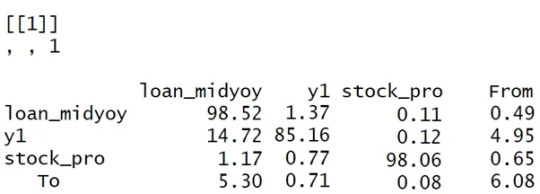
Analysis and interpretation:
Self-contribution: The fluctuations of loan_midyoy, y1, and stock_pro are mainly caused by their own shocks, which can be seen from the high percentages on their diagonals.
Mutual influence: y1 and stock_pro contribute less to each other's fluctuations, but y1 has a relatively large contribution to the fluctuations of loan_midyoy (14.72%).
System Fluctuation Impact: The “From” and “To” columns provide an overall measure of spillover effects. For example, stock_pro has a small contribution to the fluctuation of the system (0.65% comes from the impact of stock_pro), but the system has a greater impact on the fluctuation of stock_pro (6.08% of the fluctuation comes from the system).```{r} tvp.gevd.fft(fit, df, c(pi+0.00001,pi/12,0),37) ```
The same goes for Fourier transform. It is divided into those within 1 year and 1-3 years, and the sum is the previous picture.
DY I used the R language's spillover package to modify the interface.
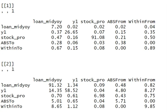
Part of the code logic:
function (ir1, h, Sigma, df) { ir10 <- list() n <- length(Sigma[, 1]) for (oo in 1:n) { ir10[[oo]] <- matrix(ncol = n, nrow = h) for (pp in 1:n) { rep <- oo + (pp - 1) * (n) ir10[[oo]][, pp] <- ir1[, rep] } } ir1 <- lapply(1:(h), function(j) sapply(ir10, function(i) i[j, ])) denom <- diag(Reduce("+", lapply(ir1, function(i) i %*% Sigma %*% t(i)))) enum <- Reduce("+", lapply(ir1, function(i) (i %*% Sigma)^2)) tab <- sapply(1:nrow(enum), function(j) enum[j, ]/(denom[j] * diag(Sigma))) tab0 <- t(apply(tab, 2, function(i) i/sum(i))) assets <- colnames(df) n <- length(tab0[, 1]) stand <- matrix(0, ncol = (n + 1), nrow = (n + 1)) stand[1:n, 1:n] <- tab0 * 100 stand2 <- stand - diag(diag(stand)) stand[1:(n + 1), (n + 1)] <- rowSums(stand2)/n stand[(n + 1), 1:(n + 1)] <- colSums(stand2)/n stand[(n + 1), (n + 1)] <- sum(stand[, (n + 1)]) colnames(stand) <- c(colnames(df), "From") rownames(stand) <- c(colnames(df), "To") stand = round(stand, 2) return(stand) }
0 notes
Text
regression-modeling-practice Course Week_3
Test a Multiple Regression Model
(Testen Sie ein multiples Regressionsmodell)
My Research:
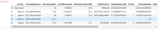
My research question was to establish the relationship and possible causality between global pollution (co2 emissions levels) and breastcancer per 100.000 female among countries. The relationship was later extended to include internet use and female employe rate among all countries.
Sample and measure
The aim of this assignment is to analysis the association and model fit among the following variables from the Gapminder dataset.
Explanatory variables – internet use rate, female employe rate, , co2 emissions
Response - Breastcancer per 100th Women
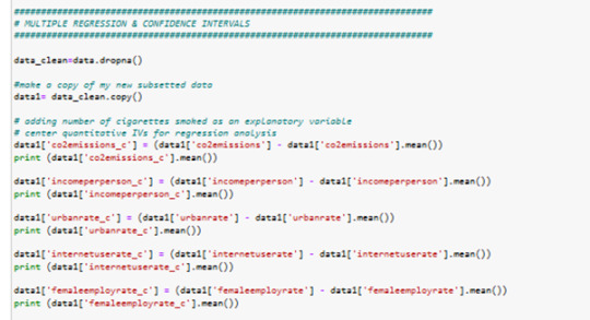
Code
all columns of interest centered...
liniar regression anaylsis between values breastcancer100th and CO2emissions centered value:
R sguared is 8%
Pvalue is 0.001
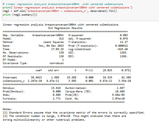
R sguared is 8%;
In fact, Co2 emissions explain only about 8% of the variability in breastcanserper100th.
So, there's clearly some error in estimating the response value with this model.
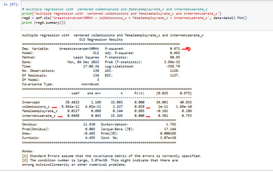
I added some other Values to my Modell
femaleemployrate and internetuserate are my new Values in my Modell
femaleemployrate has a P value0.88 >0.05
p value for femaleemployrate is not significant in this Modell
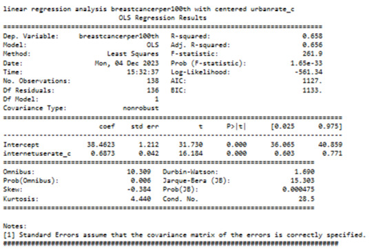
we can see that the R squared in 0.67
it means Co2 emissions + internetuserate together explain 67% of the variability in breastcanserper100th.
P value of internetuserrate is 0.001 and < 0.05
p value for internetuserate is significant in this Modell
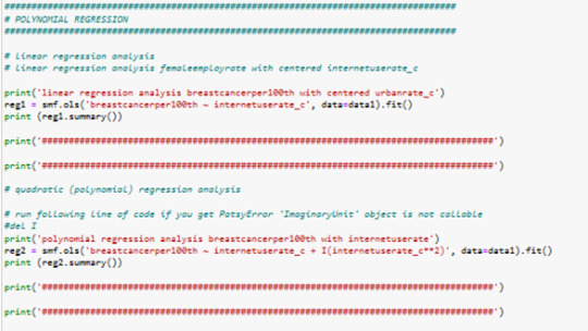
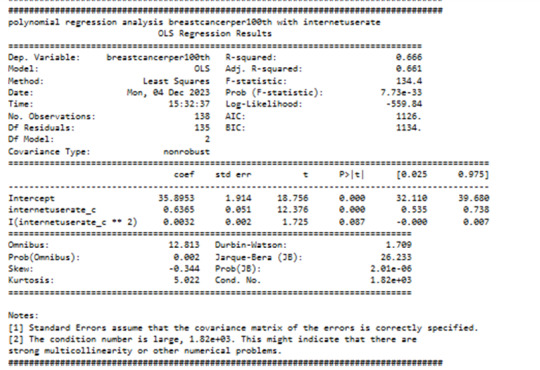
as next I have added internetuserate^2 in my Modell
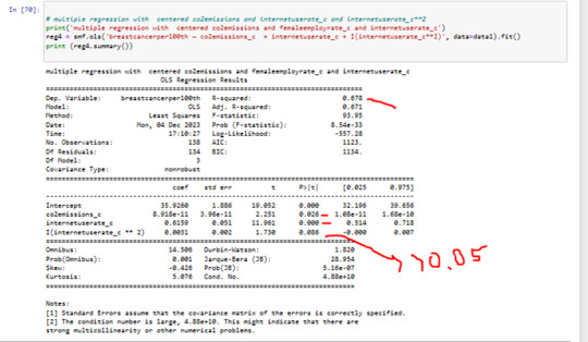
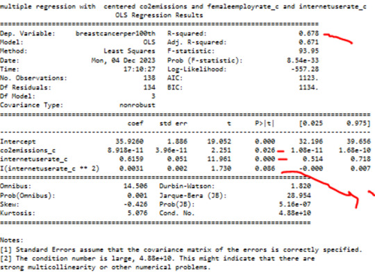
P value of quadratic term of internetuserate 0.08
.The quadratic term of internetuserate in our modell is not significant.
Plots
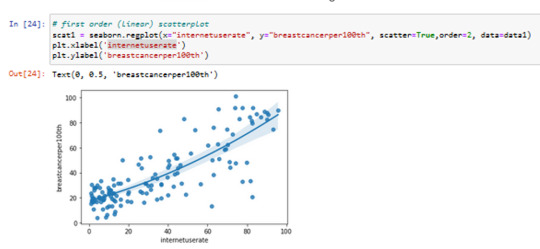
First Order scatter plot
x=internetuserate
y=breastcancerper100th

2 order scatterplot
x=internetuserate
y=breastcancerper100th
2 different modells to compare and Calculation Results
---------
Actually it was better to use linear model with internetuserate with R Value
But I have decided to use polinomial model for my further investigations to see the problems with this Modell
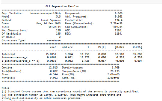
The governing beta equation is breastcancerperr100th = 33,89 + 0.5363 internateusarate_c + 0.0032 internateusarate_c**2.
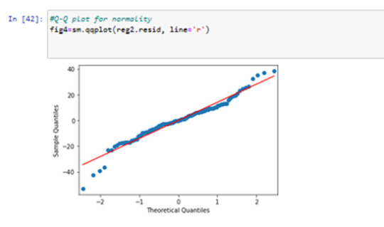
Results 8: Residual analysis
in QQ plot I can see the modell is not perfect fitting in first and last quartiles..
qq plot is not perfect normally distributed.
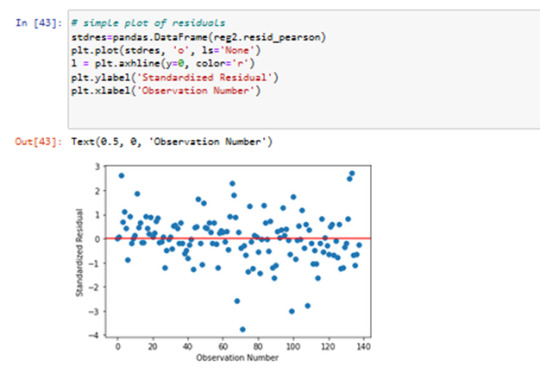
Results 9: Standardized Residual analysis
in residuals plot we can see some outliers by -3.5 standardized Reziduals..
I used standardized plot residuals, this is transformed to have a mean of 0 and standard deviation (Std) of 1. Most residuals fall within 2 Std of the mean (-2to 2). A few have more than 2 Stds (below 3 ), and below -3. For a normal distribution, I expect that 95% of the values falls within 2 stds of the mean. About 8 values fall aside this range indicating the possibility of outliers. There is only 1 extreme outlier outside 3 Stds of the mean.
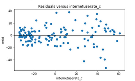
----Results 10: contribution of specific explanatory values to the model fit
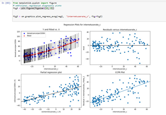
The plot in the upper right hand corner shows the residuals for
each observation at different values of Internet use rate.
There , we can see that the absolute values of the residuals
are significantly larger at higher values of Internet use rate.
But get smaller, closer to zero, as Internet use rate decreases.
I think, it' s better to use in this case only the linear modell with internetuserate.
Results 11: leverage plot analysis
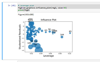
We've already identified some of these outliers in some of the other plots we've looked at, but this plot also tells us that these outliers have small or close to
zero leverage values, meaning that although they are outlying observations,
they don't have an undue influence on the estimation of the regression model.
On the other hand, we see that there are a few cases with higher average leverage.
This observation has a high leverage but is not an outlier.
(The leverage always takes on values between zero and one.)
Summary:
Conclusion
The hypothesis test shows that there is association between some of the explanatory variables CO2emissions, internet use and the response variable Breastcancer100th. The model fit better for linear regression than quadratic polynomial regression. As of now there is not enough evidence to prove causality.
0 notes
Text
Coursera Regression Modeling in Practice - Assignment week 4
Results
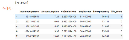
the selected response variable (lifeexpectancy from gapminder dataset) is a quantitative variable, therefore i binned that variable such that ‘1’ corresponded to the 3rd quantile and above while ‘0’ corresponded to less than the 3rd quantile, accordingly i designed the label of the new (binary) response variable as ‘life_score’ from the quantitative ‘lifeexpectancy’.
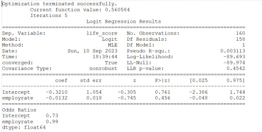
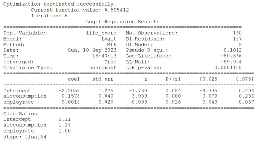
Running logistic regressions for the 4 explanatory variables i found the following evidence:
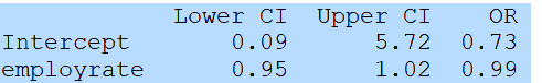
1) employrate is not associated to the response variable (life_score) since the pvalue is 0.456 and altough the OR=0.99 is slightly less than 1, the 95% Confidence Interval contains 1 therefore no probability that the employrate would impact the life_score
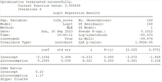
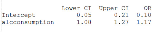
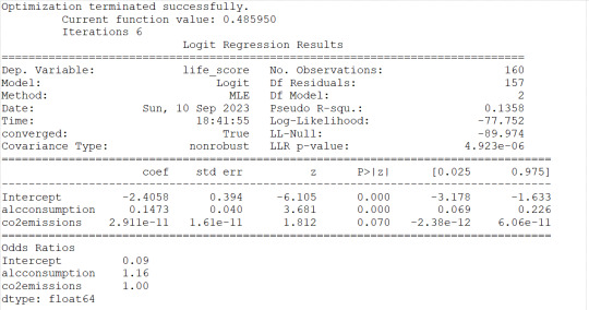
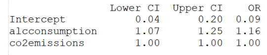
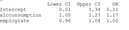
2) alcconsumption is instead significantly associated to the response variable based on the pvalue<0.0001 and the OR=1.17 with the 95%CI of 1.08 to 1.27 would indicate that people with large alcconsumption would have between 1.08 and 1.27 more probability to live longer than the 3rd quantile.
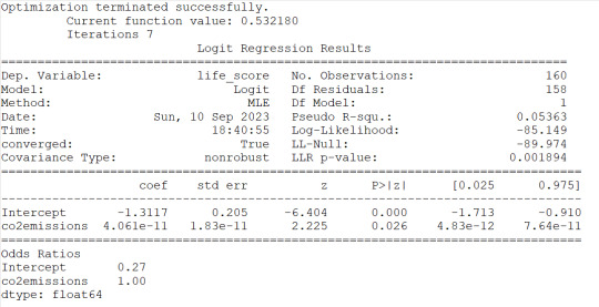
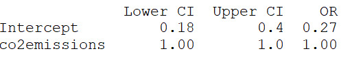
3) co2emissions seems to be associated to the response variable because of the pvof 0.026 but the OR of 1 would indicate that there is no significant impact on probability for life expectancy
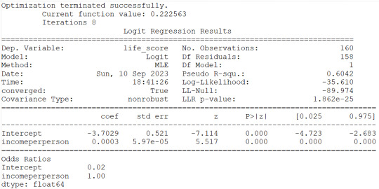
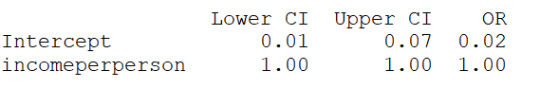
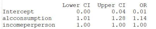
4)incomeperperson show same reesults as for co2emissions therefore same conclusions can be drawn.
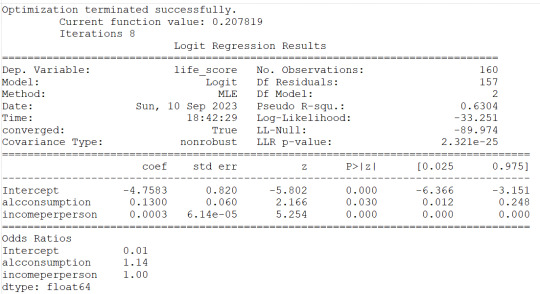
I then checked for confounding and found no evidence of it when running regression with alcconsumption and the other 3 explanatory variables as shown (in the results) by the unchanged level of significance of the alcconsumption. I can state then that the alcconsumprion is significantly associated to the life expenctancy (coeff=0.1585, pvalue<0.0001, OR=1.17, 95%IC=1.08 - 1.27 after adjusting for the other explanatory variables. Therefore people with larger alcconsumption would have 1.08 to 1.27 better propbability to live at/above the 3rd quantitle.
This result is partially supporting my hypothesis (since 1 out of 4 explanatory variables have an association with the response variable) but it is also counterintuitive to the expectation of alcohol consumption favouring longer life expectancy. Overlall this week results confirms the past week (week 3) outcome of a basically misspecified model which is missing some other important explanatory variables.
Details and code are following.
Code
import numpy
import pandas
import statsmodels.api as sm
import statsmodels.formula.api as smf
data=pandas.read_csv('gapminder.csv',low_memory=False)
data.head()
data['incomeperperson']=pandas.to_numeric(data['incomeperperson'],errors='coerce')
data['alcconsumption']=pandas.to_numeric(data['alcconsumption'],errors='coerce')
data['co2emissions']=pandas.to_numeric(data['co2emissions'],errors='coerce')
data['employrate']=pandas.to_numeric(data['employrate'],errors='coerce')
data['lifeexpectancy']=pandas.to_numeric(data['lifeexpectancy'],errors='coerce')
sub1=data[['incomeperperson','alcconsumption','co2emissions', 'employrate','lifeexpectancy']].dropna()
#binning lifeexpectancy to be 1 at and above 3rd quantile and moving to the new variable 'life_score'
v=numpy.quantile(sub1['lifeexpectancy'],[0.75])
print(v)
sub1['life_score']=['1' if x >= v else '0' for x in sub1['lifeexpectancy']]
sub1['life_score']=pandas.to_numeric(sub1['life_score'],errors='coerce')
sub1.head()
#logistic regression for employment rate
lreg1=smf.logit(formula='life_score ~ employrate', data=sub1).fit()
print(lreg1.summary())
print('Odds Ratios')
print (round(numpy.exp(lreg1.params),2))
#odd ratios with 95% conf interval
params=lreg1.params
conf=lreg1.conf_int()
conf['OR']=params
conf.columns=['Lower CI', 'Upper CI', 'OR']
print(round(numpy.exp(conf),2))
#logistic regression for alcohol consumption
lreg1=smf.logit(formula='life_score ~ alcconsumption', data=sub1).fit()
print(lreg1.summary())
print('Odds Ratios')
print (round(numpy.exp(lreg1.params),2))
#odd ratios with 95% conf interval
params=lreg1.params
conf=lreg1.conf_int()
conf['OR']=params
conf.columns=['Lower CI', 'Upper CI', 'OR']
print(round(numpy.exp(conf),2))
#logistic regression for CO2 emissions
lreg1=smf.logit(formula='life_score ~ co2emissions', data=sub1).fit()
print(lreg1.summary())
print('Odds Ratios')
print (round(numpy.exp(lreg1.params),2))
#odd ratios with 95% conf interval
params=lreg1.params
conf=lreg1.conf_int()
conf['OR']=params
conf.columns=['Lower CI', 'Upper CI', 'OR']
print(round(numpy.exp(conf),2))
#logistic regression for incomeperperson
lreg1=smf.logit(formula='life_score ~ incomeperperson', data=sub1).fit()
print(lreg1.summary())
print('Odds Ratios')
print (round(numpy.exp(lreg1.params),2))
#odd ratios with 95% conf interval
params=lreg1.params
conf=lreg1.conf_int()
conf['OR']=params
conf.columns=['Lower CI', 'Upper CI', 'OR']
print(round(numpy.exp(conf),2))
#check for confounding - adding c02emissions to alcohol consumption
lreg1=smf.logit(formula='life_score ~ alcconsumption+co2emissions', data=sub1).fit()
print(lreg1.summary())
print('Odds Ratios')
print (round(numpy.exp(lreg1.params),2))
#odd ratios with 95% conf interval
params=lreg1.params
conf=lreg1.conf_int()
conf['OR']=params
conf.columns=['Lower CI', 'Upper CI', 'OR']
print(round(numpy.exp(conf),2))
#check for confounding - adding incomeperperson to alcohol consumption
lreg1=smf.logit(formula='life_score ~ alcconsumption+incomeperperson', data=sub1).fit()
print(lreg1.summary())
print('Odds Ratios')
print (round(numpy.exp(lreg1.params),2))
#odd ratios with 95% conf interval
params=lreg1.params
conf=lreg1.conf_int()
conf['OR']=params
conf.columns=['Lower CI', 'Upper CI', 'OR']
print(round(numpy.exp(conf),2))
#check for confounding - adding employment rate to alcohol consumption
lreg1=smf.logit(formula='life_score ~ alcconsumption+employrate', data=sub1).fit()
print(lreg1.summary())
print('Odds Ratios')
print (round(numpy.exp(lreg1.params),2))
#odd ratios with 95% conf interval
params=lreg1.params
conf=lreg1.conf_int()
conf['OR']=params
conf.columns=['Lower CI', 'Upper CI', 'OR']
print(round(numpy.exp(conf),2))
0 notes
Text
Data analysis Tools: Module 3. Pearson correlation coefficient (r / r2)
According my last studies ( ANOVA and Chi square test of independence), there is a relationship between the variables under observation:
Quantitative variable: Femaeemployrate (Percentage of female population, age above 15, that has been employed during the given year)
Quantitative variable: Incomeperperson (Gross Domestic Product per capita in constant 2000 US$).
I have calculated the Pearson Correlation coefficient and I have created the graphic:
“association between Income per person and Female employ rate
PearsonRResult(statistic=0.3212540576761761, pvalue=0.015769942076727345)”
r=0.3212540576761761à It means that the correlation between female employ rate and income per person rate is positive and it is stark (near to 0)
p-value=0,015 < 0.05 it means that the is a relationship
The graphic shows the positive correlation.
In the graphic in the low range of the x axis is obserbed a different correlation, perhaps this correlation should be also analysis.
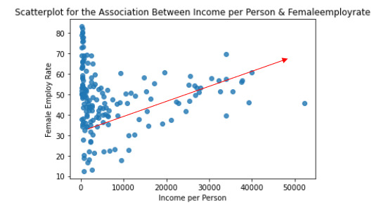
And the r2=0,32125*0,32125= 0,10
It can be predicted 10% of the variability in the rate of female employ rate according the income per person. (The fraction of the variability of one variable that can be predicted by the other).
Program:
# -*- coding: utf-8 -*-
"""
Created on Thu Aug 31 13:59:25 2023
@author: ANA4MD
"""
import pandas
import numpy
import seaborn
import scipy
import matplotlib.pyplot as plt
data = pandas.read_csv('gapminder.csv', low_memory=False)
# lower-case all DataFrame column names - place after code for loading data above
data.columns = list(map(str.lower, data.columns))
# bug fix for display formats to avoid run time errors - put after code for loading data above
pandas.set_option('display.float_format', lambda x: '%f' % x)
# to fix empty data to avoid errors
data = data.replace(r'^\s*$', numpy.NaN, regex=True)
# checking the format of my variables and set to numeric
data['femaleemployrate'].dtype
data['polityscore'].dtype
data['incomeperperson'].dtype
data['urbanrate'].dtype
data['femaleemployrate'] = pandas.to_numeric(data['femaleemployrate'], errors='coerce', downcast=None)
data['polityscore'] = pandas.to_numeric(data['polityscore'], errors='coerce', downcast=None)
data['incomeperperson'] = pandas.to_numeric(data['incomeperperson'], errors='coerce', downcast=None)
data['urbanrate'] = pandas.to_numeric(data['urbanrate'], errors='coerce', downcast=None)
data['incomeperperson']=data['incomeperperson'].replace(' ', numpy.nan)
# to create bivariate graph for the selected variables
print('relationship femaleemployrate & income per person')
# bivariate bar graph Q->Q
scat2 = seaborn.regplot(
x="incomeperperson", y="femaleemployrate", fit_reg=False, data=data)
plt.xlabel('Income per Person')
plt.ylabel('Female Employ Rate')
plt.title('Scatterplot for the Association Between Income per Person & Femaleemployrate')
data_clean=data.dropna()
print ('association between Income per person and Female employ rate')
print (scipy.stats.pearsonr(data_clean['incomeperperson'], data_clean['femaleemployrate']))
Results:
relationship femaleemployrate & income per person
association between Income per person and Female employ rate
PearsonRResult(statistic=0.3212540576761761, pvalue=0.015769942076727345)
Data analysis Tools: Module 3. Pearson correlation coefficient (r / r2)
According my last studies ( ANOVA and Chi square test of independence), there is a relationship between the variables under observation:
Quantitative variable: Femaeemployrate (Percentage of female population, age above 15, that has been employed during the given year)
Quantitative variable: Incomeperperson (Gross Domestic Product per capita in constant 2000 US$).
I have calculated the Pearson Correlation coefficient and I have created the graphic:
“association between Income per person and Female employ rate
PearsonRResult(statistic=0.3212540576761761, pvalue=0.015769942076727345)”
r=0.3212540576761761à It means that the correlation is positive and it is stark (near to 0)
p-value=0,015 < 0.05 à it means that the is a relationship
The graphic shows the positive correlation.
And the r2=0,32125*0,32125= 0,10àwe can predict 10% of the variability in the rate of female employ rate according the income per person. (The fraction of the variability of one variable that can be predicted by the other).
Program:
# -*- coding: utf-8 -*-
"""
Created on Thu Aug 31 13:59:25 2023
@author: ANA4MD
"""
import pandas
import numpy
import seaborn
import scipy
import matplotlib.pyplot as plt
data = pandas.read_csv('gapminder.csv', low_memory=False)
# lower-case all DataFrame column names - place after code for loading data above
data.columns = list(map(str.lower, data.columns))
# bug fix for display formats to avoid run time errors - put after code for loading data above
pandas.set_option('display.float_format', lambda x: '%f' % x)
# to fix empty data to avoid errors
data = data.replace(r'^\s*$', numpy.NaN, regex=True)
# checking the format of my variables and set to numeric
data['femaleemployrate'].dtype
data['polityscore'].dtype
data['incomeperperson'].dtype
data['urbanrate'].dtype
data['femaleemployrate'] = pandas.to_numeric(data['femaleemployrate'], errors='coerce', downcast=None)
data['polityscore'] = pandas.to_numeric(data['polityscore'], errors='coerce', downcast=None)
data['incomeperperson'] = pandas.to_numeric(data['incomeperperson'], errors='coerce', downcast=None)
data['urbanrate'] = pandas.to_numeric(data['urbanrate'], errors='coerce', downcast=None)
data['incomeperperson']=data['incomeperperson'].replace(' ', numpy.nan)
# to create bivariate graph for the selected variables
print('relationship femaleemployrate & income per person')
# bivariate bar graph Q->Q
scat2 = seaborn.regplot(
x="incomeperperson", y="femaleemployrate", fit_reg=False, data=data)
plt.xlabel('Income per Person')
plt.ylabel('Female Employ Rate')
plt.title('Scatterplot for the Association Between Income per Person & Femaleemployrate')
data_clean=data.dropna()
print ('association between Income per person and Female employ rate')
print (scipy.stats.pearsonr(data_clean['incomeperperson'], data_clean['femaleemployrate']))
Results:
relationship femaleemployrate & income per person
association between Income per person and Female employ rate
PearsonRResult(statistic=0.3212540576761761, pvalue=0.015769942076727345)
0 notes
Text
assignment week 4
TESTING A POTENTIAL MODERATOR
I will test the effect of taken a public or written pledge to remain a virgin until marriage in the relation between sex intercourse and duration of romantic relationship.
Data management for the moderator variable
DATA3 = sub7[(sub7["H1ID5"]== 0)]
DATA4 = sub7[(sub7["H1ID5"]== 1)]
ct3 = pd.crosstab(DATA3["lengh_class"], DATA3["H1RI27_1"])
print(ct3)
colsum= ct3.sum(axis=0)
colpct=ct3/colsum
print(colpct)
cs3= scipy.stats.chi2_contingency(ct3)
print(cs3)
ct4 = pd.crosstab(DATA4["lengh_class"], DATA4["H1RI27_1"])
print(ct4)
colsum= ct4.sum(axis=0)
colpct=ct4/colsum
print(colpct)
cs4= scipy.stats.chi2_contingency(ct4)
print(cs4)
Results
DATA3 = sub7[(sub7["H1ID5"]== 0)]
ct3 = pd.crosstab(DATA3["lengh_class"], DATA3["H1RI27_1"])
print(ct3)
H1RI27_1 1.0 2.0
lengh_class
0-2 68 67
3-5 1 2
6-10 1 1
colsum= ct3.sum(axis=0)
colpct=ct3/colsum
print(colpct)
cs3= scipy.stats.chi2_contingency(ct3)
print(cs3)
H1RI27_1 1.0 2.0
lengh_class
0-2 0.971429 0.957143
3-5 0.014286 0.028571
6-10 0.014286 0.014286
Chi2ContingencyResult(statistic=0.34074074074074073, pvalue=0.8433524060031772, dof=2, expected_freq=array([[67.5, 67.5],
[ 1.5, 1.5],
[ 1. , 1. ]]))
ct4 = pd.crosstab(DATA4["lengh_class"], DATA4["H1RI27_1"])
print(ct4)
colsum= ct4.sum(axis=0)
colpct=ct4/colsum
print(colpct)
cs4= scipy.stats.chi2_contingency(ct4)
print(cs4)
H1RI27_1 1.0 2.0
lengh_class
0-2 4 3
3-5 1 0
H1RI27_1 1.0 2.0
lengh_class
0-2 0.8 1.0
3-5 0.2 0.0
Chi2ContingencyResult(statistic=0.0, pvalue=1.0, dof=1, expected_freq=array([[4.375, 2.625],
[0.625, 0.375]]))
Interpretation: in the presence of 2 groups of potential moderator variable, the relation between sex intercourse and the duration of romantic relationship did not change. The P value remains > 0.05. We conclude that there is not association between the 2 variables independently of the fact to take a public or written pledge to remain a virgin until marriage.
0 notes
Text
week 3 assignment correlation
I want to see the correlation between the level of desapointment of adolescent father if the adolescent fall to college and high school study.
## CORELATION COEFFICIENT BETWEEN the father disappointment level if the adolescent did not graduate from college and if the adolescent did not graduate from high school.
Data management
DATA1= DATA.copy()
DATA1["H1WP15"]= DATA1["H1WP15"].replace("6",numpy.nan)
DATA1["H1WP15"]= DATA1["H1WP15"].replace("7",numpy.nan)
DATA1["H1WP15"]= DATA1["H1WP15"].replace("8",numpy.nan)
DATA1["H1WP15"]= DATA1["H1WP15"].replace("9",numpy.nan)
DATA1["H1WP16"]= DATA1["H1WP16"].replace("6",numpy.nan)
DATA1["H1WP16"]= DATA1["H1WP16"].replace("7",numpy.nan)
DATA1["H1WP16"]= DATA1["H1WP16"].replace("8",numpy.nan)
DATA1["H1WP16"]= DATA1["H1WP16"].replace("9",numpy.nan)
DATA_CLEAN= DATA1.dropna()
2) calculating the correlation
print("association between the fathers level desapointment")
print(scipy.stats.pearsonr(DATA_CLEAN["H1WP15"], DATA_CLEAN["H1WP16"]))
scat1= seaborn.regplot(x= "H1WP15", y = "H1WP16", data = DATA_CLEAN)
plt.xlabel("desapointment level college")
plt.ylabel("desapointment level high school")
plt.title("scaterplot for the association between the father level desapointment for failling college and high school")
3) Results
association between the fathers level desapointment
PearsonRResult (statistic=0.8099571461012307, pvalue=0.0)
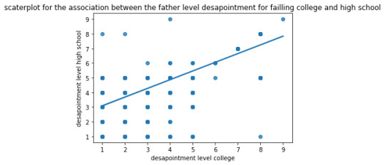
Interpretation: with a r = 0.8 and a p value of 0.0, we can conclude that the father level disappointment for failing both college and high school are strongly correlated. This correlation is positive and statistically significant.
0 notes
Text
WEEK 2 ASSIGNMENT
CHI SQUARE TEST.
ASSOCIATION BETWEEN SEX INTERCOURSE (EXPLANATORY) AND DURATION OF ROMANTIC RELATIONSHIP
## chi squarte test
import scipy.stats
ct1= pd.crosstab(sub8["lengh_class"], sub8["H1RI27_1"])
print(ct1)
colsum=ct1.sum(axis=0)
colpct=ct1/colsum
print(colpct)
print("chi square value, p value and expected counts")
cs1=scipy.stats.chi2_contingency(ct1)
print(cs1)
## Results
H1RI27_1 1.0 2.0
lengh_class
0-2 72 71
3-5 2 2
6-10 1 1
H1RI27_1 1.0 2.0
lengh_class
0-2 0.960000 0.959459
3-5 0.026667 0.027027
6-10 0.013333 0.013514
chi square value, p value and expected counts
Chi2ContingencyResult(statistic=0.0002816102816102786, pvalue=0.9998592047717735, dof=2, expected_freq=array([[71.97986577, 71.02013423],
[ 2.01342282, 1.98657718],
[ 1.00671141, 0.99328859]]))
The p value is> 0.05
we will not reject the H0. We can then conclude that there is not association between the sex intercourse and the duration of romantic relationship. the proportion of adolescents having 1 or more than one intercourse is not different in the different categories of duration are not significally different.
0 notes
Text
Congratulations, tumblr, this is not Gaussian! If we fit a Gaussian to this data, we get:
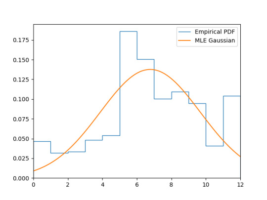
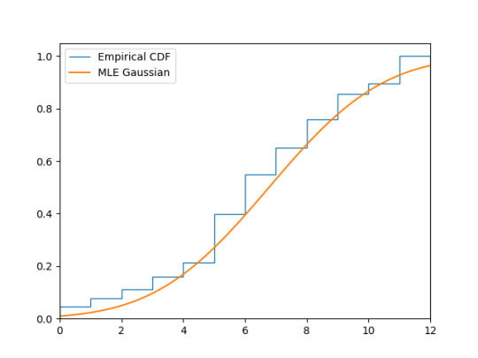
A Kolmogorov–Smirnov test produces:
KstestResult(statistic=0.15607735863481176, pvalue=6.521057734204922e-12)
That p-value is quite significant!
Source code here
#math#stats#programming#i might have slightly messed up the plotting of the empirical cdf by just using cumsum here but I trust scipy.stats for the ks test#do your civic duty#mine
107 notes
·
View notes
Photo

Who can relate??
Get this sweatshirt here! : https://rdbl.co/3fc8em9
#econ student#econ#college#university#statistical significance#statistics#econometrics#pvalue#economics#econ major#economicsblr#studyblr#econ jokes#econ memes
3 notes
·
View notes
Text
The p-value in statistics

We’ve been dancing around the p-value for some time and gave it a good definition early on. The p-value is simply the probability that you’ve made a type one error, the lower the p-value the less chance you have of making a type one error, but you increase your probability that you’ll make a type two error (errors in statistics for more). However, just like with the mean, there’s more than meets…
View On WordPress
#academia#Education#graduate school#learning#Math#mathematics#p-value#PhD#school#science#statistics#stats#pvalue
2 notes
·
View notes