#femalereality | Explore Tumblr posts and blogs

girltalkcollectives · 2 months ago

Text

Being Considered Pretty By Society's Standards Is Both A Privilege And A Prison

Pretty privilege is real. The world treats you differently when you fit society's beauty standards. Doors open easier. People are nicer. Life seems smoother.

But here's what nobody talks about - the exhausting pressure of maintaining that privilege. The constant awareness that your value seems directly tied to how you look that day.

Because that's the thing about pretty privilege - it's conditional. It's fragile. It depends on:

Staying thin enough

Looking young enough

Being polished enough

Appearing effortless enough

Always being "enough"

The world is kinder when you're pretty, but it's also watching. Waiting. Ready to revoke those privileges the moment you:

Gain weight

Show age

Look tired

Stop trying

Just exist

Pretty privilege means people listen when you speak, but they're not always hearing your words. They're looking at your face, your body, your package. Your ideas come second to your appearance.

It means getting opportunities, but always wondering if you earned them or if your face did. It means constant impostor syndrome, wondering if your achievements are yours or your looks'.

Pretty privilege means easier dating - but it also means never quite knowing if someone likes you or just likes looking at you. If they're interested in your mind or just your appearance. If they want to know you or just be seen with you.

It means being treated better at work, but also not being taken as seriously. Being called "sweetie" in meetings where men are called "sir." Having your intelligence seem surprising rather than expected.

The pressure is constant:

Don't age

Don't change

Don't slip

Don't fail

Don't rest

Because pretty privilege isn't a gift - it's a loan. One that can be recalled the moment you stop meeting the requirements. One that charges interest in the form of your self-worth.

And the maintenance? It's expensive:

Time spent on appearance

Money spent on upkeep

Energy spent on presentation

Youth spent on preservation

Worth spent on perception

Pretty privilege means being seen - but often not for who you are. Being heard - but often not for what you say. Being valued - but often not for what you offer beyond your appearance.

It means being put on a pedestal that feels more like a stage. Where everyone's watching, waiting for you to fall. Where the spotlight feels more like a searchlight, looking for flaws.

The truth about pretty privilege is:

It's temporary

It's conditional

It's expensive

It's exhausting

It's a trap

Because while the world treats pretty girls better, it also punishes them harder for stepping out of line. For aging. For changing. For being human.

So yes, pretty privilege is real. But so is pretty pressure. And maybe instead of envying the privilege or denying its existence, we need to talk about how messed up it is that someone's face determines how human they're allowed to be.

At the end of the day, pretty privilege isn't actually privilege at all. It's just another way society controls women by making their worth conditional on their appearance.

10 notes · View notes

usfvisualstudent · 8 months ago

Text

Final Project

For this final project, I knew what data set I wanted to use for it. With the increase attention on mental health, I wanted to put a focus on the suicide rates in the United States. Once I found the data set from data.gov, I wanted to address this problem. I wanted to show that there is an increase over the years and show that there needs to be a focus point on improving the overall mental health in the United States.

Code:

install.packages("ggplot2") library("ggplot2") MaleRates <- c(21.2, 20, 19.8, 19.9, 19.8, 20.4, 20.4, 20.9, 21.1, 21.9, 21.7, 21.2, 21, 21.5, 21.2, 20.5, 20.7, 20.5, 20.3, 19.8, 19.1, 18.9, 17.8, 17.7, 18.2, 18.5, 18.1, 18.1, 18.1, 18.1, 18.5, 19, 19.2, 19.8, 20, 20.4, 20.3, 20.7, 21.1, 21.4, 22.4, 22.8) FemaleRates <- c(5.6, 5.6, 7.4, 5.7, 6, 5.8, 5.5, 5.6, 5.2, 5.5, 5.3, 5.1, 4.9, 4.8, 4.7, 4.6, 4.6, 4.4, 4.3, 4.3, 4.3, 4.3, 4, 4, 4.1, 4.2, 4.2, 4.5, 4.4, 4.5, 4.6, 4.8, 4.8, 5, 5.2, 5.4, 5.5, 5.8, 6, 6, 6.1, 6.2) AllRates <- c(13.2, 12.5, 13.1, 12.2, 12.3, 12.5, 12.4, 12.6, 12.5, 13, 12.8, 12.5, 12.3, 12.5, 12.3, 12, 12.1, 11.9, 11.8, 11.5, 11.2, 11.1, 10.5, 10.4, 10.7, 10.9, 10.8, 11, 10.9, 11, 11.3, 11.6, 11.8, 12.1, 12.3, 12.6, 12.6, 13, 13.3, 13.5, 14, 14.2) years <- c(1950, 1960, 1970, 1980, 1981, 1982, 1983, 1984, 1985, 1986, 1987, 1988, 1989, 1990, 1991, 1992, 1993, 1994, 1995, 1996, 1997, 1998, 1999, 2000, 2001, 2002, 2003, 2004, 2005, 2006, 2007, 2008, 2009, 2010, 2011, 2012, 2013, 2014, 2015, 2016, 2017, 2018) Rates = data.frame(years, MaleRates, FemaleRates, AllRates) Rates1 = data.frame(years, MaleRates) Rates2 = data.frame(years, FemaleRates) ggplot(data = Rates, aes(x = years, group = 2)) + geom_line(aes(y = MaleRates, color = "Male"), size = 1.2) + geom_line(aes(y = FemaleRates, color = "Female"), size = 1.2) + geom_line(aes(y = AllRates, color = "All"), size = 1.2) + labs(title = "Suicide Rates in the United States Over the Years", x = "Years", y = "Rates") + scale_color_manual(values = c("Male" = "darkblue", "Female" = "pink", "All" = "orange")) + theme_minimal()

Output:

0 notes

usfstatstudent · 1 year ago

Text

Final project

Topic: Death rates for suicide, by sex, race, Hispanic origin, and age: United States

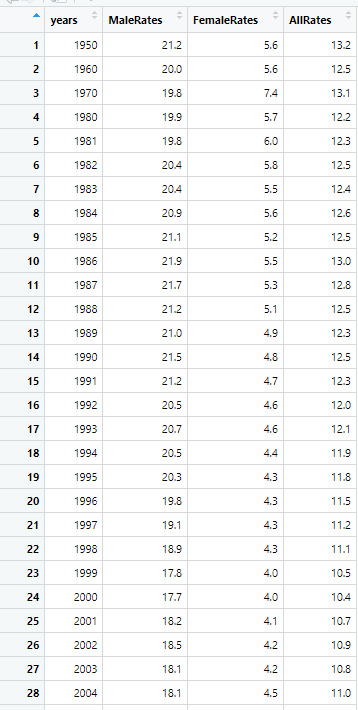
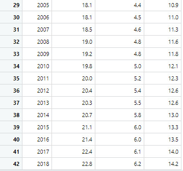
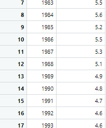
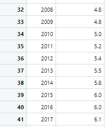
For my final project, I wanted to do something that I thought was important. As the topic of mental health issues continue to become a more and more talked about issues, I wanted to focus on death rates of suicide in the United States. The data set I used I found on data.gov, this data set categorizes by sex, race, Hispanic origin, age and total. For this project, I chose to focus on the sex category and see if the suicide rates were higher in males or females.

Dataset: This table shows the rates of male and females and the combined rates of both genders.

Source: https://catalog.data.gov/dataset/death-rates-for-suicide-by-sex-race-hispanic-origin-and-age-united-states-020c1

2. To start with my hypothesis, My hypothesis are:

H0: There is no difference between male and female suicide rates in the United States.

H1: There is a difference between male and female suicide rates in the United States.

3. Sample

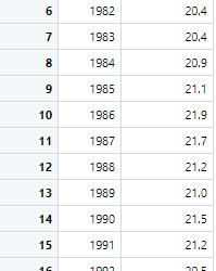
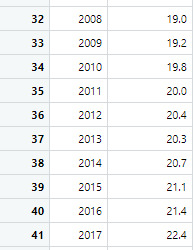
The first sample is the male suicide rates and the second sample is the female suicide rates

4. Code in R Studio

MaleRates <- c(21.2, 20, 19.8, 19.9, 19.8, 20.4, 20.4, 20.9, 21.1, 21.9, 21.7, 21.2, 21, 21.5, 21.2, 20.5, 20.7, 20.5, 20.3, 19.8, 19.1, 18.9, 17.8, 17.7, 18.2, 18.5, 18.1, 18.1, 18.1, 18.1, 18.5, 19, 19.2, 19.8, 20, 20.4, 20.3, 20.7, 21.1, 21.4, 22.4, 22.8) FemaleRates <- c(5.6, 5.6, 7.4, 5.7, 6, 5.8, 5.5, 5.6, 5.2, 5.5, 5.3, 5.1, 4.9, 4.8, 4.7, 4.6, 4.6, 4.4, 4.3, 4.3, 4.3, 4.3, 4, 4, 4.1, 4.2, 4.2, 4.5, 4.4, 4.5, 4.6, 4.8, 4.8, 5, 5.2, 5.4, 5.5, 5.8, 6, 6, 6.1, 6.2) AllRates <- c(13.2, 12.5, 13.1, 12.2, 12.3, 12.5, 12.4, 12.6, 12.5, 13, 12.8, 12.5, 12.3, 12.5, 12.3, 12, 12.1, 11.9, 11.8, 11.5, 11.2, 11.1, 10.5, 10.4, 10.7, 10.9, 10.8, 11, 10.9, 11, 11.3, 11.6, 11.8, 12.1, 12.3, 12.6, 12.6, 13, 13.3, 13.5, 14, 14.2) years <- c(1950, 1960, 1970, 1980, 1981, 1982, 1983, 1984, 1985, 1986, 1987, 1988, 1989, 1990, 1991, 1992, 1993, 1994, 1995, 1996, 1997, 1998, 1999, 2000, 2001, 2002, 2003, 2004, 2005, 2006, 2007, 2008, 2009, 2010, 2011, 2012, 2013, 2014, 2015, 2016, 2017, 2018) Rates = data.frame(years, MaleRates, FemaleRates, AllRates) Rates1 = data.frame(years, MaleRates) Rates2 = data.frame(years, FemaleRates)

t.test(MaleRates, FemaleRates)

i. The sample means: MaleRates = 20.047619 and FemaleRates = 5.066667

ii. P-value = 0.00000000000000022

iii. Significance value of a = 0.05. P-value <= Significance level.

iv. 0.00000000000000022 <= 0.05. Since the p value is less than or equal to the significance level it indicates a significant difference between the two means.

This is the code for the line chart:

ggplot(data = Rates, aes(x = years, group = 2)) + geom_line(aes(y = MaleRates, color = "Male"), size = 1.2) + geom_line(aes(y = FemaleRates, color = "Female"), size = 1.2) + geom_line(aes(y = AllRates, color = "All"), size = 1.2) + labs(title = "Suicide Rates in the United States Over the Years", x = "Years", y = "Rates") + scale_color_manual(values = c("Male" = "blue", "Female" = "red", "All" = "green")) + theme_minimal()

5. Conclusion

There is a significant difference between the two sample means, and P-value <= Significance level, therefore I can conclude the the alterative hypothesis is true.

There is a significance difference in the male suicide rate and the female suicide rate in the United States.

0 notes

rbem-amo · 2 years ago

Text

Module 3: Making Data Management Decision

Step 1: Program

""" Created on Wed Feb 22 17:51:13 2023

@author: ANA4MD """

import pandas import numpy

data = pandas.read_csv ('gapminder.csv', low_memory=False) print ('gapminder file: rows & columns') print (len(data)) #number of observations (rows) print (len(data.columns)) # number of variables (columns)

lower-case all DataFrame column names - place after code for loading data above

data.columns = list(map(str.lower, data.columns))

bug fix for display formats to avoid run time errors - put after code for loading data above

pandas.set_option('display.float_format', lambda x:'%f'%x)

checking the format of my variables

data['femaleemployrate'].dtype data['polityscore'].dtype data['incomeperperson'].dtype data['urbanrate'].dtype data['femaleemployrate'] = pandas.to_numeric(data['femaleemployrate'], errors = 'coerce', downcast=None) data['polityscore'] = pandas.to_numeric(data['polityscore'], errors = 'coerce', downcast=None) data['incomeperperson'] = pandas.to_numeric(data['incomeperperson'], errors = 'coerce', downcast=None) data['urbanrate'] = pandas.to_numeric(data['urbanrate'], errors = 'coerce', downcast=None)

splits femaleemployrate into 9 groups (10-20, 20-30, …80-90), creating a new variable femalerate

print('distribution for female employ rate , splits into 9 groups and with a new variable femalerate') data['femalerate'] = pandas.cut(data['femaleemployrate'], [10, 20, 30, 40, 50, 60, 70, 80, 90]) c5 = data['femalerate'].value_counts(sort=False, dropna=True) print (c5) print('distribution in 9 groups for female employ rate in %') p5 = data['femalerate'].value_counts(sort=False, dropna=False, normalize=True) print (p5)

splits into 6 groups -considering very poor. poor, low class, midle class, upper class, rich, creating a new variable income

print('distribution for income per person splits into 6 groups and creating a new variable income') data['income'] = pandas.cut(data['incomeperperson'], [0, 1000, 2000, 6000, 24000, 60000, 120000]) c6 = data['income'].value_counts(sort=False, dropna=False) print (c6) print('distribution in 6 groups for income per person in %') p6 = data['income'].value_counts(sort=False, dropna=False, normalize=True) print (p6)

splits urbanrate into 9 groups (10-20, 20-30, …80-90), creating a new variable urban

print('distribution for urban rate, splits into 9 groups and a new variable urban') data['urban'] = pandas.cut(data['urbanrate'], [10, 20, 30, 40, 50, 60, 70, 80, 90]) c7 = data['urban'].value_counts(sort=False, dropna=True) print (c7) print('distribution in 9 groups for urban in %') p7 = data['urban'].value_counts(sort=False, dropna=False, normalize=True) print (p7)

crosstabs evaluating which % were put into which femalerate

print('cross check of female employ rate by using crosstab') print (pandas.crosstab(data['femalerate'], data['femaleemployrate']))

print('Study the income per person distribution considering more or less demacraty and different female employ rate')

subgroup countries with less democraty <0 & employ rate >70%

sub3=data[(data['polityscore']<=0) & (data['femaleemployrate']>70)]

make a copy of my new subsetted data

sub4 = sub3.copy()

income frequency for subgroup less democraty <0 & employ rate >70%

print('distribution for income per person in % considering countries with less democraty <0 & female employ rate >70%') p8 = sub4['income'].value_counts(sort=False, dropna=False, normalize=True) print (p8)

subgroup countries more democraty >0 & employ rate >70%

sub5=data[(data['polityscore']>=0) & (data['femaleemployrate']>70)]

make a copy of my new subsetted data

sub6 = sub5.copy()

income frequency for subgroup more democraty >0 & employ rate >70%

print('distribution for income per person in % considering countries with more democraty >0 & female employ rate >70%') p9 = sub6['income'].value_counts(sort=False, dropna=False, normalize=True) print (p9)

print('Study the distribution of urban rate considering the female employ rate')

subgroup countries employ rate >70%

sub7=data[(data['femaleemployrate']>70)]

make a copy of my new subsetted data

sub8 = sub7.copy()

urban rate frequency for subgroup employ rate >70%

print('distribution of urban rate with female employ rate >70%') p10 = sub8['urban'].value_counts(sort=False, dropna=False) print (p10)

subgroup countries employ rate <=30%

sub9=data[(data['femaleemployrate']<=30)]

make a copy of my new subsetted data

sub10 = sub9.copy()

polity score frequency for subgroup employ rate <=30%

print('distribution of urban rate with female employ rate <=30%') p11 = sub10['urban'].value_counts(sort=False, dropna=False) print (p11)

print('Study the income per person in categories considering countries with more and less democraty and different female employ rate')

new inc variable, in 6 categories

def inc (row): if row['incomeperperson'] < 1000 : return 'very poor' if row['incomeperperson'] < 2000 : return 'poor' if row['incomeperperson'] < 6000 : return 'Low class' if row['incomeperperson'] < 24000 : return 'midle class' if row['incomeperperson'] < 60000 : return 'upper class' if row['incomeperperson'] < 120000 : return 'rich'

data['inc'] = data.apply (lambda row: inc (row),axis=1) print('distribution of income per person in 6 categories') c14 = data['inc'].value_counts(sort=False, dropna=True) print(c14) print('distribution of income per person in 6 categories in %') p14 = data['inc'].value_counts(sort=False, dropna=True, normalize=True) print(p14)

subgroup countries more democraty >0 & employ rate >70%

sub11=data[(data['polityscore']<=0) & (data['femaleemployrate']>70)]

make a copy of my new subsetted data

sub12 = sub11.copy()

income frequency for subgroup more democraty >0 & employ rate >70%

print('distribution for income per person categories in % considering countries with more democraty >0 & femmale employ rate >70%') c15 = sub12['inc'].value_counts(sort=False, dropna=False, normalize=True) print (c15)

print('Study the polity score distribution considering the female employ rate %')

subset data to female employ rate betwenn >30% y <70%

sub13=data[(data['femaleemployrate']>=30) & (data['femaleemployrate']<70)]

make a copy of my new subsetted data

sub14 = sub13.copy() print ('counts for original polityscore') c16 = data['polityscore'].value_counts(sort=False) print(c16) print ('counts for polityscore and female employ rate betwenn 30% & 70%') c17 = sub14['polityscore'].value_counts(sort=False, dropna=False) print(c17)

subset data to female employ rate <30%

sub17=data[(data['femaleemployrate']<30)]

make a copy of my new subsetted data

sub18 = sub17.copy() print('counts for polityscore and female employ rate <30%') c19 = sub18['polityscore'].value_counts(sort=False, dropna=False) print(c19)

subset data to female employ rate >70%

sub19=data[(data['femaleemployrate']>70)]

make a copy of my new subsetted data

sub20 = sub19.copy() print('counts for polityscore and female employ rate >70%') c20 = sub20['polityscore'].value_counts(sort=False, dropna=False) print(c20)

print('study female employ rate distribution considering urban rate')

subset data to urban rate <30%

sub21=data[(data['urbanrate']<30)]

make a copy of my new subsetted data

sub22 = sub21.copy() print('counts for female employ rate considering urban rate <30%') c21 = sub22['femalerate'].value_counts(sort=False, dropna=False) print(c21)

subset data to urban rate >70%

sub23=data[(data['urbanrate']>70)]

make a copy of my new subsetted data

sub24 = sub23.copy() print('counts for female employ rate considering urban rate >70%') c22 = sub24['femalerate'].value_counts(sort=False, dropna=False) print(c22)

subset data to urban rate >70%

sub23=data[(data['urbanrate']<=70 + (data['urbanrate']>=30))]

make a copy of my new subsetted data

sub24 = sub23.copy() print('counts for female employ rate considering urban rate between 30% & 70%') c22 = sub24['femalerate'].value_counts(sort=False, dropna=False) print(c22)

print('study female employ rate distribution considering income per person')

subset data to income per person <1000

sub25=data[(data['incomeperperson']<1000)]

make a copy of my new subsetted data

sub26 = sub25.copy() print('counts for female employ rate considering income per personn <1000') c23 = sub25['femalerate'].value_counts(sort=False, dropna=False) print(c23)

subset data to income per person <2000

sub27=data[(data['incomeperperson']<2000)]

make a copy of my new subsetted data

sub28 = sub27.copy() print('counts for female employ rate considering income per personn <2000') c24 = sub28['femalerate'].value_counts(sort=False, dropna=False) print(c24)

subset data to income per person >24000

sub29=data[(data['incomeperperson']>24000)]

make a copy of my new subsetted data

sub30 = sub29.copy() print('counts for female employ rate considering income per personn >24000') c25 = sub30['femalerate'].value_counts(sort=False, dropna=False) print(c25)

subset data to income per person between 2000 y 24000

sub31=data[(data['incomeperperson']>2000 + (data['incomeperperson']<24000))]

make a copy of my new subsetted data

sub32 = sub31.copy() print('counts for female employ rate considering income per person between 2000 & 24000') c26 = sub32['femalerate'].value_counts(sort=False, dropna=False) print(c26)

Step 2: Results

gapminder file: rows & columns 213 16 distribution for female employ rate , splits into 9 groups and with a new variable femalerate (10, 20] 7 (20, 30] 11 (30, 40] 34 (40, 50] 50 (50, 60] 46 (60, 70] 19 (70, 80] 8 (80, 90] 3 Name: femalerate, dtype: int64 distribution in 9 groups for female employ rate in % (10.0, 20.0] 0.032864 (20.0, 30.0] 0.051643 (30.0, 40.0] 0.159624 (40.0, 50.0] 0.234742 (50.0, 60.0] 0.215962 (60.0, 70.0] 0.089202 (70.0, 80.0] 0.037559 (80.0, 90.0] 0.014085 NaN 0.164319 Name: femalerate, dtype: float64 distribution for income per person splits into 6 groups and creating a new variable income (0.0, 1000.0] 54 (1000.0, 2000.0] 26 (2000.0, 6000.0] 46 (6000.0, 24000.0] 39 (24000.0, 60000.0] 22 (60000.0, 120000.0] 3 NaN 23 Name: income, dtype: int64 distribution in 6 groups for income per person in % (0.0, 1000.0] 0.253521 (1000.0, 2000.0] 0.122066 (2000.0, 6000.0] 0.215962 (6000.0, 24000.0] 0.183099 (24000.0, 60000.0] 0.103286 (60000.0, 120000.0] 0.014085 NaN 0.107981 Name: income, dtype: float64 distribution for urban rate, splits into 9 groups and a new variable urban (10, 20] 13 (20, 30] 22 (30, 40] 24 (40, 50] 22 (50, 60] 24 (60, 70] 34 (70, 80] 24 (80, 90] 21 Name: urban, dtype: int64 distribution in 9 groups for urban in % (10.0, 20.0] 0.061033 (20.0, 30.0] 0.103286 (30.0, 40.0] 0.112676 (40.0, 50.0] 0.103286 (50.0, 60.0] 0.112676 (60.0, 70.0] 0.159624 (70.0, 80.0] 0.112676 (80.0, 90.0] 0.098592 NaN 0.136150 Name: urban, dtype: float64 cross check of female employ rate by using crosstab femaleemployrate 11.300000 12.400000 … 82.199997 83.300003 femalerate … (10, 20] 1 1 … 0 0 (20, 30] 0 0 … 0 0 (30, 40] 0 0 … 0 0 (40, 50] 0 0 … 0 0 (50, 60] 0 0 … 0 0 (60, 70] 0 0 … 0 0 (70, 80] 0 0 … 0 0 (80, 90] 0 0 … 1 1

[8 rows x 153 columns] Study the income per person distribution considering more or less demacraty and different female employ rate distribution for income per person in % considering countries with less democraty <0 & female employ rate >70% (0, 1000] 1.000000 (1000, 2000] 0.000000 (2000, 6000] 0.000000 (6000, 24000] 0.000000 (24000, 60000] 0.000000 (60000, 120000] 0.000000 Name: income, dtype: float64 distribution for income per person in % considering countries with more democraty >0 & female employ rate >70% (0, 1000] 1.000000 (1000, 2000] 0.000000 (2000, 6000] 0.000000 (6000, 24000] 0.000000 (24000, 60000] 0.000000 (60000, 120000] 0.000000 Name: income, dtype: float64 Study the distribution of urban rate considering the female employ rate distribution of urban rate with female employ rate >70% (10, 20] 5 (20, 30] 3 (30, 40] 3 (40, 50] 0 (50, 60] 0 (60, 70] 0 (70, 80] 0 (80, 90] 0 Name: urban, dtype: int64 distribution of urban rate with female employ rate <=30% (10, 20] 0 (20, 30] 1 (30, 40] 2 (40, 50] 2 (50, 60] 2 (60, 70] 5 (70, 80] 4 (80, 90] 2 Name: urban, dtype: int64 Study the income per person in categories considering countries with more and less democraty and different female employ rate distribution of income per person in 6 categories poor 26 Low class 46 midle class 39 upper class 22 very poor 54 rich 3 Name: inc, dtype: int64 distribution of income per person in 6 categories in % poor 0.136842 Low class 0.242105 midle class 0.205263 upper class 0.115789 very poor 0.284211 rich 0.015789 Name: inc, dtype: float64 distribution for income per person categories in % considering countries with more democraty >0 & femmale employ rate >70% very poor 1.000000 Name: inc, dtype: float64 Study the polity score distribution considering the female employ rate % counts for original polityscore 0.000000 6 9.000000 15 2.000000 3 -2.000000 5 8.000000 19 5.000000 7 10.000000 33 -7.000000 12 7.000000 13 3.000000 2 6.000000 10 -4.000000 6 -1.000000 4 -3.000000 6 -5.000000 2 1.000000 3 -6.000000 3 -9.000000 4 4.000000 4 -8.000000 2 -10.000000 2 Name: polityscore, dtype: int64 counts for polityscore and female employ rate betwenn 30% & 70% 9.000000 13 2.000000 1 -2.000000 4 8.000000 18 5.000000 5 10.000000 33 -7.000000 8 NaN 19 7.000000 11 3.000000 2 -4.000000 4 -1.000000 1 0.000000 2 -5.000000 2 6.000000 9 -6.000000 2 -9.000000 4 1.000000 2 -3.000000 3 4.000000 4 -10.000000 1 -8.000000 1 Name: polityscore, dtype: int64 counts for polityscore and female employ rate <30% 0.000000 2 -3.000000 2 -7.000000 3 7.000000 2 9.000000 1 -6.000000 1 -8.000000 1 5.000000 1 -10.000000 1 -4.000000 2 NaN 1 -2.000000 1 Name: polityscore, dtype: int64 counts for polityscore and female employ rate >70% 0.000000 2 6.000000 1 2.000000 1 1.000000 1 -1.000000 3 -7.000000 1 5.000000 1 -3.000000 1 Name: polityscore, dtype: int64 study female employ rate distribution considering urban rate counts for female employ rate considering urban rate <30% (10.0, 20.0] 0 (20.0, 30.0] 1 (30.0, 40.0] 3 (40.0, 50.0] 4 (50.0, 60.0] 8 (60.0, 70.0] 5 (70.0, 80.0] 6 (80.0, 90.0] 2 NaN 6 Name: femalerate, dtype: int64 counts for female employ rate considering urban rate >70% (10.0, 20.0] 3 (20.0, 30.0] 3 (30.0, 40.0] 8 (40.0, 50.0] 18 (50.0, 60.0] 18 (60.0, 70.0] 3 (70.0, 80.0] 0 (80.0, 90.0] 0 NaN 11 Name: femalerate, dtype: int64 counts for female employ rate considering urban rate between 30% & 70% (10.0, 20.0] 4 (20.0, 30.0] 8 (30.0, 40.0] 23 (40.0, 50.0] 31 (50.0, 60.0] 28 (60.0, 70.0] 16 (70.0, 80.0] 8 (80.0, 90.0] 3 NaN 19

Name: femalerate, dtype: int64 study female employ rate distribution considering income per person counts for female employ rate considering income per personn <1000 (10.0, 20.0] 2 (20.0, 30.0] 2 (30.0, 40.0] 7 (40.0, 50.0] 7 (50.0, 60.0] 14 (60.0, 70.0] 9 (70.0, 80.0] 8 (80.0, 90.0] 3 NaN 2 Name: femalerate, dtype: int64 counts for female employ rate considering income per personn <2000 (10.0, 20.0] 4 (20.0, 30.0] 3 (30.0, 40.0] 11 (40.0, 50.0] 17 (50.0, 60.0] 16 (60.0, 70.0] 12 (70.0, 80.0] 8 (80.0, 90.0] 3 NaN 6 Name: femalerate, dtype: int64 counts for female employ rate considering income per personn >24000 (10.0, 20.0] 0 (20.0, 30.0] 0 (30.0, 40.0] 1 (40.0, 50.0] 5 (50.0, 60.0] 13 (60.0, 70.0] 2 (70.0, 80.0] 0 (80.0, 90.0] 0 NaN 4 Name: femalerate, dtype: int64 counts for female employ rate considering income per person between 2000 & 24000 (10.0, 20.0] 2 (20.0, 30.0] 7 (30.0, 40.0] 20 (40.0, 50.0] 29 (50.0, 60.0] 28 (60.0, 70.0] 6 (70.0, 80.0] 0 (80.0, 90.0] 0 NaN 18 Name: femalerate, dtype: int64

Step 3: Interpretation

After analysis of the distributions and frequencies for all the combination, following assessments can be done:

The distribution for female employ rate >70% & <30% is similar for countries with more and with less democracy. Polity score looks like no impact in the female employ rate.

For countries with urban rate>70% the distribution of female employ rate is very similar in all the groups. In case of countries with urban rate <30% the female employ rate is more concentrated in the groups from 30% to 60% and for rest of countries with urban rates between 30% and 70% the female employ rate distribution is concentrated in countries with urban rate between 30% and 70%. Urban rate looks like no impact in the female employ rate.

The female employ rate in case of income per person less than 2000 has a distribution in all groups, but in case of income per person more than 24000 the distribution is concentrated between 40% and 60%. The distribution for rest of countries with incoming between 2000 y 24000 has a concentration between 305 and 60%. The income per person could be a factor for the female employ rate.

0 notes