#data_set

[edujournalblogs]

Master Program in Data Analytics and Data Science

Do you have a natural instinct to make sense of raw numbers? If so, then this should be the right field for you. You should be passionate of finding insights from data set, using mathematical and statistical tools, basic probability, python libraries like panda and numpy, data visualization libraries like tableau, algorithms in machine learning, MySql, basic Natural Language processing (nlp) etc. You learn all the tools, solve a bunch of problems, work on real-time projects and build a strong portfolio of work.

Understanding the problem is mandatory (algorithms in machine language), so is data cleaning and restructuring data (transformation). it is estimated that only 20% is utilized for algorithm and remaining 80% for data cleaning ie., data errors, redundant entries. If you don't have clean data, all the models you have built are all garbage.

People from non-technical backgrounds have made their way through to become Data Analyst and then Data Scientist. It is a challenging career. Companies care only about your skills and nothing else.

URL : https://www.edujournal.com/masters-program-in-data-analytics-data-science

[grotechminds]

Data-Driven Testing with Selenium and Python

Data-Driven Testing with Selenium and Python

In the realm of test automation, the ability to execute tests with different sets of data is a game-changer. Data-driven testing allows testers to run the same test scenario with multiple inputs, making scripts more versatile and efficient. When it comes to Selenium test automation testing with Python, harnessing the power of data-driven testing can significantly enhance the effectiveness of your test suites.

Understanding Data-Driven Testing:

Data-driven testing is an approach where test scripts are designed to run with multiple sets of data. Instead of hardcoding values within the script, data-driven testing separates the test logic from the test data. This approach offers several advantages, including:

Versatility: The same test script can be executed with different input data.

Scalability: Easily scale test suites by adding more data sets.

Maintainability: Changes to test data don't require modifications to the test script.

Implementing Data-Driven Testing with Selenium and Python:

Let's explore how to implement data-driven testing using Selenium and Python. We'll use a simple example of a login functionality to demonstrate the concept.

1. Data Preparation:

Create a separate file or data source containing the test data. This can be a CSV file, Excel sheet, or even a Python list or dictionary.

python

Copy code

# Example data in a Python list

login_data = [

 {"username": "user1", "password": "pass1"},

 {"username": "user2", "password": "pass2"},

 # Add more data sets as needed

]

2. Test Script Modification:

Modify the test script to read test data from the external source. Here, we use a simple loop to iterate through the data sets and perform the login test.

python

Copy code

from selenium import webdriver

# Assuming login_data is defined as mentioned above

def test_login():

 driver = webdriver.Chrome()

 for data_set in login_data:

 username = data_set["username"]

 password = data_set["password"]

 # Your login test steps using Selenium

 driver.get("login_page_url")

 driver.find_element_by_id("username").send_keys(username)

 driver.find_element_by_id("password").send_keys(password)

 driver.find_element_by_id("login_button").click()

 # Add assertions or verifications as needed

 driver.quit()

3. Parameterized Testing with Pytest:

Using a testing framework like Pytest makes parameterized testing even more straightforward. Pytest's @pytest.mark.parametrize decorator allows you to easily iterate through different data sets.

python

Copy code

import pytest

# Assuming login_data is defined as mentioned above

@pytest.mark.parametrize("username, password", [(d["username"], d["password"]) for d in login_data])

def test_login(username, password):

 driver = webdriver.Chrome()

 # Your login test steps using Selenium

 driver.get("login_page_url")

 driver.find_element_by_id("username").send_keys(username)

 driver.find_element_by_id("password").send_keys(password)

 driver.find_element_by_id("login_button").click()

 # Add assertions or verifications as needed

 driver.quit()

Best Practices for Data-Driven Testing:

Separate Test Data from Test Logic:

Keep test data in external files or sources, ensuring easy updates without modifying the test script.

Handle Data Variations:

Include diverse data sets to cover different scenarios and edge cases.

Logging and Reporting:

Implement comprehensive logging to capture data-driven test execution details.

Randomize Data Order:

Randomizing the order of test data sets helps identify any dependencies between data sets.

Handle Data-Driven Frameworks:

Consider implementing more sophisticated data-driven frameworks for larger projects, such as using a database to store test data.

Conclusion:

Data-driven testing is a potent strategy to maximize the efficiency and coverage of your Selenium test scripts in Python. Whether you're enrolled in a Selenium Python course or independently exploring automation testing with Python, incorporating data-driven principles will undoubtedly elevate your testing capabilities.

By embracing the versatility of data-driven testing, you pave the way for scalable and maintainable test suites, making your Selenium Python Automation Testing with cucumber framework.

[hardik20sharma]

Peer-graded Assignment: Running Your First Program

The program I have written (in Python):

import pandas as p import numpy as n

data_set = p.read_csv('Modified_DataSet.csv', low_memory = False) print("\nRows in data set: ", len(data_set))            # Number of rows in data set print("Cols in data set: ", len(data_set.columns))    # Number of cols in data set

state_count = data_set["State"].value_counts(sort=False) state_count_percentage = data_set["State"].value_counts(sort=False, normalize=True)

print("\nDistribution of patients in each state: ", end="\n\n") print(state_count)

print("\nDistribution of patients in each state (in %): ", end="\n\n") print(state_count_percentage * 100)

gender_count = data_set["Gender"].value_counts(sort=False) gender_count_percentage = data_set["Gender"].value_counts(sort=False, normalize=True)

print("\nGender distribution of patients: ", end="\n\n") print(gender_count)

print("\nGender distribution of patients (in %): ", end="\n\n") print(gender_count_percentage * 100)

Output of the program:

Rows in data set:  40493 Cols in data set:  3

Distribution of patients in each state:

Bihar                                        6994 Mizoram                                        19 Andaman and Nicobar Islands                     7 Puducherry                                      5 West Bengal                                    24 Arunachal Pradesh                               2 Odisha                                        268 Rajasthan                                      41 Chandigarh                                    316 Andhra Pradesh                                417 Ladakh                                          6 Chhattisgarh                                   17 Nagaland                                        7 Manipur                                       114 Jammu and Kashmir                              14 Sikkim                                          2 Uttarakhand                                    40 Dadra and Nagar Haveli and Daman and Diu       27 Gujarat                                      2662 Assam                                           6 Karnataka                                    8350 Himachal Pradesh                                9 Punjab                                         51 Haryana                                        16 Telangana                                      49 Tamil Nadu                                  20562 Kerala                                        237 Maharashtra                                    83 Meghalaya                                       1 Uttar Pradesh                                  62 Goa                                             6 Madhya Pradesh                                 25 Delhi                                          46 Jharkhand                                       7 Tripura                                         1 Name: State, dtype: int64

Distribution of patients in each state (in %):

Bihar                                       17.272121 Mizoram                                      0.046922 Andaman and Nicobar Islands                  0.017287 Puducherry                                   0.012348 West Bengal                                  0.059270 Arunachal Pradesh                            0.004939 Odisha                                       0.661843 Rajasthan                                    0.101252 Chandigarh                                   0.780382 Andhra Pradesh                               1.029808 Ladakh                                       0.014817 Chhattisgarh                                 0.041983 Nagaland                                     0.017287 Manipur                                      0.281530 Jammu and Kashmir                            0.034574 Sikkim                                       0.004939 Uttarakhand                                  0.098783 Dadra and Nagar Haveli and Daman and Diu     0.066678 Gujarat                                      6.573976 Assam                                        0.014817 Karnataka                                   20.620848 Himachal Pradesh                             0.022226 Punjab                                       0.125948 Haryana                                      0.039513 Telangana                                    0.121009 Tamil Nadu                                  50.779147 Kerala                                       0.585286 Maharashtra                                  0.204974 Meghalaya                                    0.002470 Uttar Pradesh                                0.153113 Goa                                          0.014817 Madhya Pradesh                               0.061739 Delhi                                        0.113600 Jharkhand                                    0.017287 Tripura                                      0.002470 Name: State, dtype: float64

Gender distribution of patients:

M    27128 F    13365 Name: Gender, dtype: int64

Gender distribution of patients (in %):

M    66.994295 F    33.005705 Name: Gender, dtype: float64

Conclusion:

From the given data we can analyse-

Approx 67% of the patients are Male and 33% of the patients are female

Found out that more than 50% of the cases come from Tamil Nadu

The state least affected is Meghalaya.

[datapheonixx-blog]

#Data _hidden_trends_Observation

Data_set chosen for analysis and research is from gapminder.

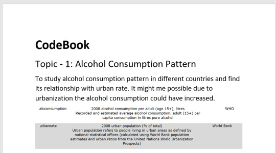
Topic_Discovery_on: Alcohol Consumption associating with employment rate.

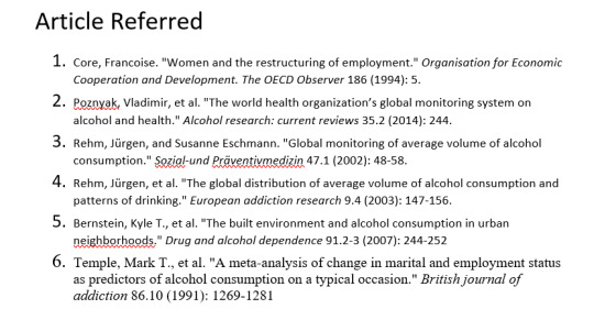
Variables a.k.a predictors chosen are mentioned in image one & two.

Hypothesis@ impact on alcohol intake trends due to employment .

The insights i was able to draw from the topics i searched for the above mentioned variables are:- the alcohol consumption was measured as per capita consumption and average volume of consumption were divided on the basis of gender and age. Alcohol consumption worldwide is contributing to develop as one of big health concerns, as it is responsible for 3 million deaths each year and often cause disability among the age group of 15 to 49; in males, heavy drinkers account for 7.1 % global disease burden, exceeding that of female by approx 4.9%. In the paper “the built environment and alcohol consumption in urban neighborhood” conducted a survey of NYC inhabitants gathering information to understand their neighborhood of residence and studying the  alcohol consumption pattern of the city, to find a correlation.  The meta data analysis survey was done on marital and employment status with alcohol consumption, to understand the effect of heavy alcohol consumption. The marriage separation, was accompanied by heavy drinking, the major key feature which was lacking was analyzing jointly male and female drinkers, in order to derive child parenting efficiency, which has been neglected. The references are mentioned in the form of MLA citations in third image. So, my study will be focusing towards deriving relation between alcohol consumption in urban areas and change in trends of alcohol consumption due to employment rate across the globe. While i was finding research articles or work done previously on employment rate and female employ rate, many new topics arise and mostly related to fertility causing change in female employment, or employment trends suffering due to non-equality in past decades.

[kasier01]

Assignment 2

i start by importing the data_set

after i verify my number of obervation and column

an then i calculted the frequancy distrubution of my 2 variable

1)alccomsumption

2) life expentancy

and to finish i select my variable that i'm going to use and remove it in the data_set

forming a new data_set df1

[hajnalkafilepcoursera]

Week 4 - Creating graphs

The previous weeks I was investigating if the polity score has influence on the life expectancy rate and suicide rate.

This week I used a filter to sort out only those rows, where the life expectancy is below 55 years. To not influence the frequency table, I also sorted out the empty fields.

I created 2 new variables: 1 - Age groups: 48-50, 51-53, 54-55. 2 - Polity groups: originally it goes from -10 to 10, but I wanted to create 4 groups for easier overview. Autocrata: -10 to -6. Slightly autocrata: -5 to 0. Slightly democrata: 1 to 5. Democrata: 6 to 10.

The dataset I used: gapminder.csv

Findings: I have created 2 bar charts. 1: Univariate bar chart according to polity groups. Since this is a categorical variable I had to use the 'describe' function to see the top, frequency, count and unique values. You can see the results and the bar chart below. The 'Slightly Autocrata' group has the most values between the age group of 48-55 years. I would assume that the most values would be coming from the 'Autocrata' group with -6 to -10 polity score, but this is not the case right now.

2. Bivariate bar chart. For this one I used the original polity scores (not the grouped values). So my x-axis is the polity score, the y-axis is the count. This is a bivariate bar chart, the higher points are at -1 and 6-7 polity scores. I also used the describe function for this barchart, which you can see below.

My code:

-- coding: utf-8 --

""" Created on Mon Oct 17 15:12:49 2022

@author: FIH4HTV """

import pandas import numpy import seaborn import matplotlib.pyplot as plt

data = pandas.read_csv('Data_Sets/gapminder.csv', low_memory=False)

data['lifeexpectancy'].dtype

#setting variables to numeric

data['lifeexpectancy'] = pandas.to_numeric(data['lifeexpectancy'], errors="coerce") data['polityscore'] = pandas.to_numeric(data['polityscore'], errors="coerce") data['suicideper100th'] = pandas.to_numeric(data['suicideper100th'], errors="coerce")

#setting filter for data to show me only those data where the expected life is =<55 yrs

sub1 = data[(data['lifeexpectancy'] <= 55)]

#make a copy of your filtered data

sub2 = sub1.copy()

#SETTING MISSING DATA: empty cells, drop not a number values

sub2['lifeexpectancy'] = sub2['lifeexpectancy'].replace(' ', numpy.nan) sub2['polityscore'] = sub2['polityscore'].replace(' ', numpy.nan) sub2['suicideper100th'] = sub2['suicideper100th'].replace(' ', numpy.nan)

#new variables for life expectancy, create less age groups

#age: 48-50 is group1, 51-54: group2, 55-58: group3

recode1 ={48.398: '48-50', 48.397: '48-50', 48.132: '48-50', 48.196: '48-50', 48.673: '48-50', 48.718: '48-50', 49.025: '48-50', 50.411: '48-50', 49.553: '48-50', 50.239: '48-50', 51.093: '51-53', 51.088: '51-53', 51.444: '51-53', 51.219: '51-53', 51.384: '51-53', 51.610: '51-53', 51.879: '51-53', 53.183: '51-53', 52.797: '51-53', 54.097: '54-55', 54.210: '54-55', 54.116: '54-55', 54.675: '54-55', 47.794: '48-50'} sub2['agegroup']=sub2['lifeexpectancy'].map(recode1)

#name your table

print('Counts of Age groups at birth')

#count of variables to show

c1 = sub2['agegroup'].value_counts(sort=False) print(c1)

#show it in percentage

print('Percent of Age groups at birth') p1 = sub2['agegroup'].value_counts(sort=False, normalize=True) print(p1)

#new variables for polity score, create less groups: 1-4

#polity score: from -10 to -6: group1, from -5 to 0: group2, from 1 to 5: group3, from 6 to 10: group:4

recode2 ={-10: 'Autocrata', -9: 'Autocrata', -8: 'Autocrata', -7: 'Autocrata', -6: 'Autocrata', -5: 'Slightly Autocrata', -4: 'Slightly Autocrata', -3: 'Slightly Autocrata', -2: 'Slightly Autocrata', -1: 'Slightly Autocrata', 0: 'Slightly Autocrata', 1: 'Slightly Democrata', 2: 'Slightly Democrata', 3: 'Slightly Democrata', 4: 'Slightly Democrata', 5: 'Slightly Democrata', 6: 'Democrata', 7: 'Democrata', 8: 'Democrata', 9: 'Democrata', 10: 'Democrata'} sub2['politygroup']=sub2['polityscore'].map(recode2)

#count of variables to show

#new variable name! how many cases I have with the new polity group variants

print('Count of Polity group') c3 = sub2['politygroup'].value_counts(sort=False) print(c3)

#show it in percentage

print('Percent of polity group') p3 = sub2['politygroup'].value_counts(sort=False, normalize=True) print(p3)

#univariate barchart for polity group

seaborn.countplot(x="politygroup", data=sub2)

plt.xlabel('Polity groups')

plt.title('Polity groups according to life expectancy rate between 48-55 years at birth')

#standard deviation asnd other descriptive statistics for categorical variables

print('Describe polity groups')

desc1 = sub2['politygroup'].describe()

print(desc1)

#bivariate barchart

seaborn.countplot(x="polityscore", data=sub2) plt.xlabel('Polity score') plt.title('Polity scores according to life expectancy rate between 48-55 years at birth')

print('Describe polity scores') desc2 = sub2['polityscore'].describe() print(desc2)

[assignment--1]

import pandas

# Statics DATA_SET = ‘gapminder.csv’

# GapMinder indicators GP_COUNTRY = 'country’ GP_INCOMEPERPERSON = 'incomeperperson’ GP_CO2EMISSIONS = 'co2emissions’ GP_URBANRATE = 'urbanrate’

def load_data_set(filename):   print('Loading data set “’ + filename + ’”…’)   # low_memory=False prevents pandas to try to determine the data type of each value   return pandas.read_csv(filename, low_memory=False)

def load_gapminder_data_set():   "“”   Load the GapMinder data set and prepare the columns needed.   "“”   data = load_data_set(DATA_SET)

  # The number of observations   print(“Number of records: ” + str(len(data)))

  # The number of variables   print(“Number of columns: ” + str(len(data.columns)))

  # convert the values of co2emissions, urbanrate and incomeperperson to numeric   data[GP_CO2EMISSIONS] = data[GP_CO2EMISSIONS].convert_objects(convert_numeric=True)   data[GP_URBANRATE] = data[GP_URBANRATE].convert_objects(convert_numeric=True)   data[GP_INCOMEPERPERSON] = data[GP_INCOMEPERPERSON].convert_objects(convert_numeric=True)   return data

def groupby(data_set, variables):    counts = data_set.groupby(variables).size()   return counts, counts * 100 / len(counts)

def print_distributions(data, variable):   "“”   Prints the distribution of the values of a specific variable.   @param data: the data set to examine.   @param variable: the variable of interest.   "“”   distribution = groupby(data, variable)

  print(“Counts for ” + variable + “:”)   print(distribution[0])   print(“Percentages for ” + variable + “:”)   print(distribution[1])   print(” distributions “)

if __name__ == ”__main__“:   data = load_gapminder_data_set()   print_distributions(data, GP_CO2EMISSIONS)   print_distributions(data, GP_URBANRATE)   print_distributions(data, GP_INCOMEPERPERSON)

Sep 10th, 2020

MORE YOU MIGHT LIKE

Data management for the missing data week 3

IF S4BQ1=9 then S4BQ1=.;

IF S4BQ2=9 then S4BQ2=.;

IF S4BQ3C=9 then S4BQ3C=.;

IF S4BQ4C=9 then S4BQ4C=.;

label S4BQ1=“Blood/Natural Father Ever Depressed”

S4BQ2=“Blood/Natural Mother Ever Depressed”

S4BQ3C=“Any Full Bothers Ever Depressed”

S4BQ4C=“Any Full Sisters Ever Depressed”

#data management for the secondary variables

#data management for Parents

IF S4BQ1=1 or S4BQ2=1 THEN parents=“1”;

IF S4BQ1=2 or S4BQ2=2 THEN Parents=“2”;

IF S4BQ1=9 or S4BQ2=9 THEN Parents=“3”;

#data management for sibilings

IF S4BQ3C=1 or S4BQ4C=1 THEN siblings=“1”; IF S4BQ3C=2 or S4BQ4C=2 THEN siblings=“2”; IF S4BQ3C=9 or S4BQ4C=9 THEN siblings=“3”;

#data management for on*/ /*one means one of the family#IF S4BQ1=1 or S4BQ2=1 or S4BQ3C=1 or S4BQ4C=1 then one=“1”; IF S4BQ1=2 or S4BQ2=2 or S4BQ3C=2 or S4BQ4C=2 then one=“2”; IF S4BQ1=9 or S4BQ2=9 or S4BQ3C=9 or S4BQ4C=9 then one=“3”;

[yashtron]

Data Management and Visualization week 2

The second assignment of the course Data Management and Visualization is to write a program in SAS or Python and to perform univariate analysis on the variables I choose in my research for the association between CO2 emissions and urbanization.

I wrote two different posts that cover this weeks assignment. The first post is: Univariate Analysis. Here you can find the results of the analysis including the frequency distribution of the three variables (co2emissions, urban rate and income per person) of my study and the output of my Python program.

The second post, Distributions with Python, explains the Python program I wrote. The complete program can be seen here.

#!/usr/bin/env python3 # -*- coding: utf-8 -*- import pandas # Statics DATA_SET = 'gapminder.csv' # GapMinder indicators GP_COUNTRY = 'country' GP_INCOMEPERPERSON = 'incomeperperson' GP_CO2EMISSIONS = 'co2emissions' GP_URBANRATE = 'urbanrate' def load_data_set(filename):    """    Loads a data set from the file system ��  @param filename: the name of the CSV file that contains the data set    """    print('Loading data set "' + filename + '"...')    # low_memory=False prevents pandas to try to determine the data type of each value    return pandas.read_csv(filename, low_memory=False) def load_gapminder_data_set():    """    Load the GapMinder data set and prepare the columns needed.    """    data = load_data_set(DATA_SET)        # The number of observations    print("Number of records: " + str(len(data)))        # The number of variables    print("Number of columns: " + str(len(data.columns)))    # convert the values of co2emissions, urbanrate and incomeperperson to numeric    data[GP_CO2EMISSIONS] = data[GP_CO2EMISSIONS].convert_objects(convert_numeric=True)    data[GP_URBANRATE] = data[GP_URBANRATE].convert_objects(convert_numeric=True)    data[GP_INCOMEPERPERSON] = data[GP_INCOMEPERPERSON].convert_objects(convert_numeric=True)    return data     def groupby(data_set, variables):    """    Get the distributed values of a variable of the data_set.    @param data_set: the data set to examine.    @param variables: the variable, or list of variables, of interest.    @return a tuple of 2 pandas.core.series.Series objects where the first            object is the absolute distribution over the values of            the given variable(s) and the second list is their            precentages as part of the total number of rows.    """    counts = data_set.groupby(variables).size()    return counts, counts * 100 / len(counts) def print_distributions(data, variable):    """    Prints the distribution of the values of a specific variable.    @param data: the data set to examine.    @param variable: the variable of interest.    """    distribution = groupby(data, variable)        print("Counts for " + variable + ":")    print(distribution[0])    print("Percentages for " + variable + ":")    print(distribution[1])    print("----------------------------") if __name__ == "__main__":    data = load_gapminder_data_set()    print_distributions(data, GP_CO2EMISSIONS)    print_distributions(data, GP_URBANRATE)    print_distributions(data, GP_INCOMEPERPERSON)

[codersarea-blog]

Visualizing Data

data = pd.read_csv("C:\Users\Sai Kumar\PycharmProjects\Data Analysis\data_sets\nesarc_pds.csv", low_memory=False)

#bug fix pd.set_option('display.float_format', lambda x:'%f'%x)

#setting variables to numeric data['TAB12MDX'] = pd.to_numeric(data['TAB12MDX']) data['CHECK321'] = pd.to_numeric(data['CHECK321']) data['S3AQ3B1'] = pd.to_numeric(data['S3AQ3B1']) data['S3AQ3C1'] = pd.to_numeric(data['S3AQ3C1']) data['AGE'] = pd.to_numeric(data['AGE'])

#subset data to young adults age 18 to 25 who have smoked in the past 12 months sub1=data[(data['AGE']>=18) & (data['AGE']<=25) & (data['CHECK321']==1)]

#make a copy of my new subsetted data sub2 = sub1.copy()

SETTING MISSING DATA

recode missing values to python missing (NaN)

sub2['S3AQ3B1'] = sub2['S3AQ3B1'].replace(9, np.nan)

recode missing values to python missing (NaN)

sub2['S3AQ3C1'] = sub2['S3AQ3C1'].replace(99, np.nan)

recode1 = {1: 6, 2: 5, 3: 4, 4: 3, 5: 2, 6: 1} sub2['USFREQ'] = sub2['S3AQ3B1'].map(recode1)

recode2 = {1: 30, 2: 22, 3: 14, 4: 5, 5: 2.5, 6: 1} sub2['USFREQMO'] = sub2['S3AQ3B1'].map(recode2)

A secondary variable multiplying the number of days smoked/month and the approx number of cig smoked/day

sub2['NUMCIGMO_EST'] = sub2['USFREQMO'] * sub2['S3AQ3C1']

univariate bar graph for categorical variables

First hange format from numeric to categorical

sub2["TAB12MDX"] = sub2["TAB12MDX"].astype('category')

sns.countplot(x="TAB12MDX", data=sub2) plt.xlabel('Nicotine Dependence past 12 months') plt.title('Nicotine Dependence in the Past 12 Months Among Young Adult Smokers in the NESARC Study')

outputs:

[y-yagi]

minitest-data というgemを作った

test-unitにはdataメソッドというデータ駆動テストのためのメソッドがあります(詳細は Ruby用単体テストフレームワークtest-unitでのデータ駆動テストの紹介 - ククログ(2013-01-23) 参照)。

大変便利で是非minitestでも使いたいのですが、minitest/testには同様の機能はありません。探したところ同じような機能を提供しているgemも無さそうでした。無いのなら作れば良いじゃないか、という事で作りました。

名前のまんまで、minitest/testでdataメソッドが使えるようになります。コードはこちら。

data("empty string" => [true, ""], "plain string" => [false, "hello"]) def test_empty(data) expected, target = data assert_equal(expected, target.empty?) end

test-unitのdataメソッドのインターフェイスが大変わかりやすかったので大分参考にさせて頂いています。というかまんまです。なので、blockを指定する事も出来ます。

data do data_set = {} data_set["empty string"] = [true, ""] data_set["plain string"] = [false, "hello"] data_set end def test_empty(data) expected, target = data assert_equal(expected, target.empty?) end

細かな挙動の確認が出来てないのですが、多分動いている気がします。ただ、minitestに無い機能を強引に入れ込んだので、モンキーパッチだらけです。それでも宜しければお試し下さい。

[wandersong]

How Save/Data Management Works In Wandersong

Wandersong is a musical adventure game about a bard, and it has a lot of characters and cutscenes and conversations! As a result of this, there are a LOT of very small bits of information the game needs to keep track of... The most common being, “how many times have I talked to this character?” It seems like a pointlessly small thing to write about, but it comes up a lot and I have a solution for it that I very much like, so I figured I’d share.

A typical conversation

In short: all data is stored into a giant dictionary. At the start of a new game it’s completely empty, and entries are added as the player interacts with things. If an entry doesn’t exist in the dictionary yet, it’s treated as being set to 0.

Sounds stupid simple, right? OK, it is. But it’s powerful! What follows is an explanation of how it’s implemented in GameMaker Studio.

Instead of “dictionaries,” GameMaker has a data structure called a map. For the uninitiated: a dictionary/map contains data stored in pairs, a “key” and a “value.” The “key” is kind of like an entry name or label, and the “value” tells you what it’s set to right now. At the start of the game, I make a blank map like this:

And then I have but two scripts that deal with this data.

data_set

Which takes two arguments, an entry name and a value. It either adds a new entry to the dictionary, or updates it if it already exists... and for good measure, it autosaves the game too, because why not. (Actually I forgot it did that until now, but I guess it happens so fast I never noticed, so...?)

and data_get

You give it an entry name, and it tells you what’s stored there. Or 0 if it doesn’t exist yet. (This is important!)

And here is how it typically would get used, in the interact-with-a-character event:

So for this event, I used an entry called “talking_to_bob”. I check what’s stored there, give you a different piece of dialog depending on what it is, and then set it to something new for next time. Typically in Wandersong, an NPC conversation tree follows the logic (conversation 1) - > (conversation 2) -> (conversation 3) -> (conversation 2) -> (conversation 3) -> etc. But you can do whatever you want with this. 

There are a couple big advantages here. When I save the game, I just save the contents of the game_data dictionary--which is just a couple lines of code to do--but that’s flexible enough to include any amount of data, forever. So I can add new conversations, new conversation branches, or track anything I want anytime while I’m in the middle of writing a scene, and I don’t have to worry about bookkeeping anywhere else. It lets me be flexible and loose and have weird ideas as I’m going, and it makes it very easy to add new responsive content. It’s considered bad practice to save data under a string name as I do here, since I could easily typo “talking_to_bob” and there would be no easy way to track errors that stem from that (unlike a variable name, where a typo would just make game crash). But that “talking_to_bob” entry name is not written out ANYWHERE ELSE IN THE CODE except right here, so it’s easy to correct errors. 

The other advantage is the synergy this has with my cutscene system. Or really, the way it deals with my system’s biggest weakness. This is going to be a little abstract. The weakness is this: I send instructions for an entire cutscene all at once to the scene manager, and then sit and wait for the entire scene to play out over time. This is mostly great, but what if I want the cutscene to change depending on data that gets altered after it already started... like in this one, where you enter your name and it's read back to you?

To make this work, when the cutscene instructions are sent off, instead of supplying the player name, I supply a dictionary entry to look at for the player name... this way, as the cutscene is running,the text can update as the dictionary entry updates. In GameMaker, crucially, you can’t use a regular old variable this way... 

And that... covers it! It's not as glamorous as my last how-to, but I think the usefulness is actually much broader. With all my tools and systems, I’m always looking to get the most power and flexibility with the minimal amount of typing and actual organization/management. If you’re going to make an entire game by yourself, especially one that’s overfilled with content, you have to think this way or you’ll never be done! Anyways. I hope this is useful to you. Feel free to send me questions if I left something unclear!

[dialogueschannel]

Video Interview with Phil Boyer, Senior Associate Crosslink Capital

[hardik20sharma]

Peer graded Assignment: Creating graphs for your data

The program I have written :-

import pandas as p import numpy as n import seaborn as sb import matplotlib.pyplot as plt

data_set = p.read_csv('Modified_DataSet.csv', low_memory = False) print("\nRows in data set: ", len(data_set))            # Number of rows in data set print("Cols in data set: ", len(data_set.columns))    # Number of cols in data set

state_count = data_set["State"].value_counts(sort=False) state_count_percentage = data_set["State"].value_counts(sort=False, normalize=True)

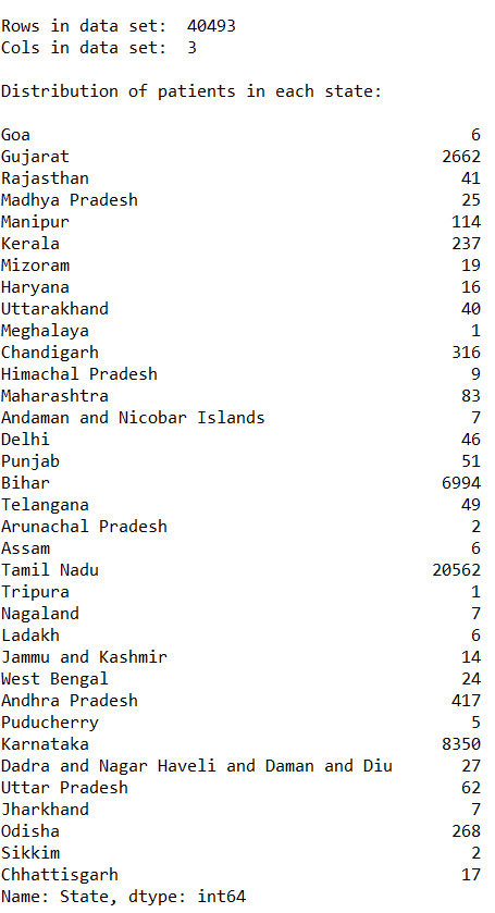
print("\nDistribution of patients in each state: ", end="\n\n") print(state_count)

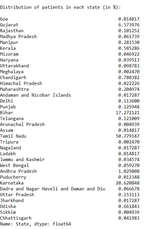
print("\nDistribution of patients in each state (in %): ", end="\n\n") print(state_count_percentage * 100)

gender_count = data_set["Gender"].value_counts(sort=False) gender_count_percentage = data_set["Gender"].value_counts(sort=False, normalize=True)

print("\nGender distribution of patients: ", end="\n\n") print(gender_count)

print("\nGender distribution of patients (in %): ", end="\n\n") print(gender_count_percentage * 100)

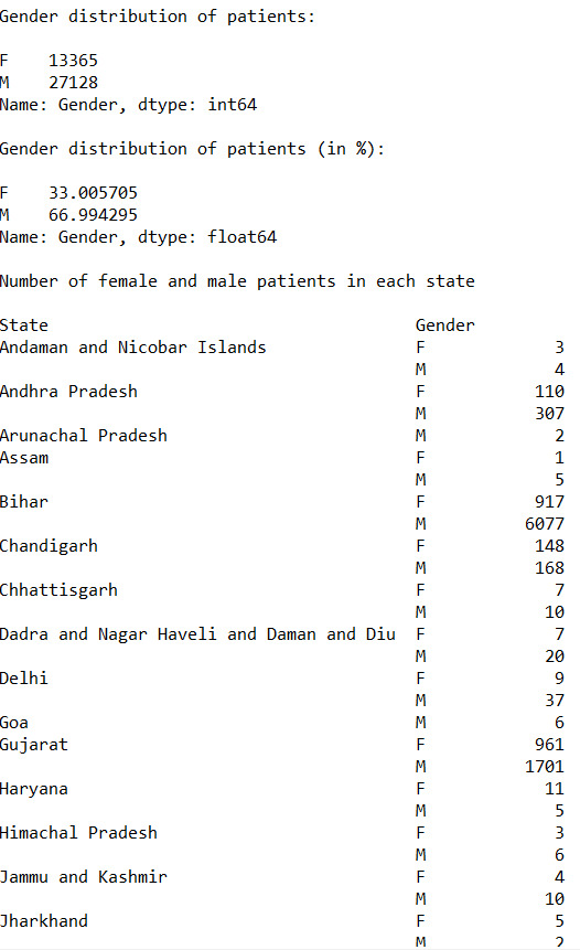
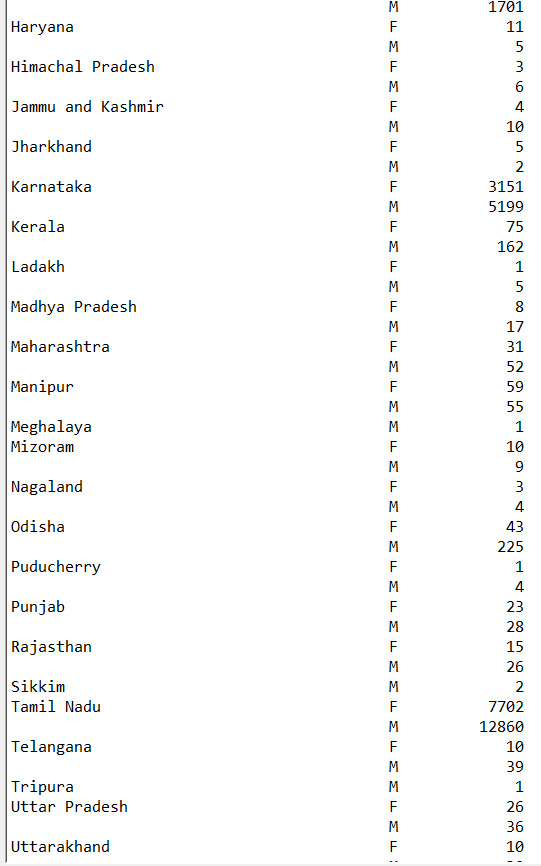
s1 = p.DataFrame(data_set).groupby(["State", "Gender"]) states_gender_distribution = s1.size() print("\nNumber of female and male patients in each state", end="\n\n") p.set_option("display.max_rows", None) print(states_gender_distribution)

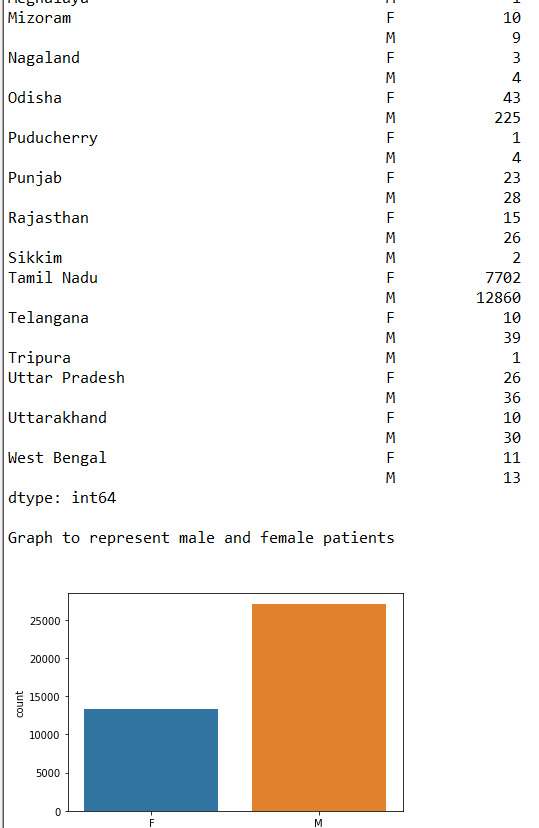
print("\nGraph to represent male and female patients", end="\n\n") data_set["Gender"] = data_set["Gender"].astype("category") sb.countplot(x="Gender",data = data_set)

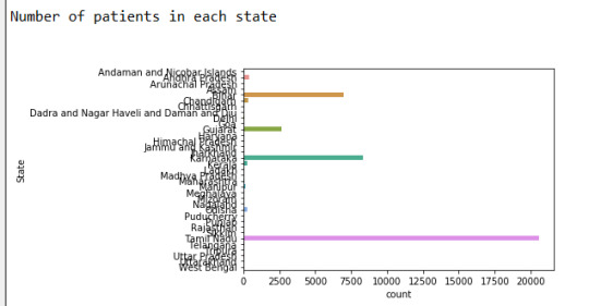
print("\nNumber of patients in each state", end="\n\n") data_set["State"] = data_set["State"].astype("category") sb.countplot(y="State",data = data_set)

Output of the program :-

1)

2)

3)

4)

5)

6)

 Conclusion :-

From the given data we can analyse-

Approx 67% of the patients are Male and 33% of the patients are female

Found out that more than 50% of the cases come from Tamil Nadu

The state least affected is Meghalaya.

We found the count of male and females patients for each state.

Successfully expressed the data through graphs.

[artofstorytelling]

Lasso: Credit Card Fraud Detection Data Set – Kaggle.com

Due to the nature of the data set column names are anonymous.  This data set was obtained from Kaggle.com, “Credit Card Fraud Detection” for the purpose of performing a lasso regression analysis.  The data set consisted of 30 predictors, all quantitative variables. These variables were transformed using PCA to conceal sensitive information.  This variable reduction technique combined like predictors in accordance to their magnitude of variance.  As such, standardization was used to effectively utilize the lasso algorithm.  

The data consisted of European credit card transactions over a two day period. A binary response variable, Class, used 1 to indicate fraud and 0 to indicate no fraud.  

A 60/40 split was used to create a train and a test set respectively.  285K records existed, 171K train and 114K test. Additional steps also included a five-fold cross validation (CV) to improve the generalization error. Given the rarity of detecting fraud, CV allowed data to be divided into five partitions taking the mean of the partition to quantify performance prior to using unseen data.  

Of the 30 variables, 29 were designated for model usage.  Positive coefficients signified an association with fraudulent activity while negative coefficients indicated no association with fraudulent activity.   More than 56% of the variables were negatively associated with the response variable (see Figure 1.). Surprisingly, Time (seconds elapsed between transactions) was negatively associated with fraudulent activity. V2, V4 and V11 were considered the most importance variables for identifying fraud.  

                                         Figure 1. Shrinkage of Coefficients

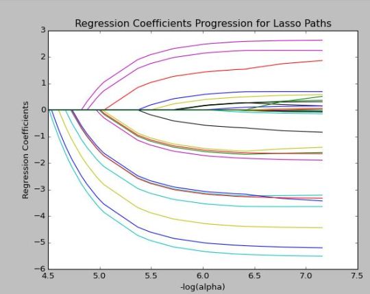
The model only explained 50% of the variance.  However, results were consistent across train and test sets with an R-Squared of 0.5 and 0.53 respectively. Train and test errors were also consistent.  

                      Table 1.  R-Squared and Mean Squared Error Table

Given the uniqueness of the data set, predictive accuracy may have been hampered by the large number of variables used in the model. PCA transformation was used prior to incorporating lasso.  This technique may have tempered a limitation of lasso in arbitrarily selecting correlated predictors. Additional improvements may require human intervention.  

Appendix: Python Code

Created on Thu Jan  5 18:32:06 2017 @author: whitfie """ #clear screen def cls():    print ('\n' * 100)

#from pandas import Series, DataFrame import pandas as pd import numpy as np import matplotlib.pylab as plt from sklearn.cross_validation import train_test_split from sklearn.linear_model import LassoLarsCV

#Load the dataset input_file =  "C:/Users/whitfie/Desktop/Python_anaconda/data_set/creditcardfraud/creditcard.csv"

#create data frame credit = pd.read_csv(input_file)

#upper-case all DataFrame column names credit.columns = map(str.upper, credit.columns)

#shuffle all rows and return in random order credit=credit.sample(frac=1)

#omit na credit_clean = credit.dropna()

credit_clean.describe()

# predictors features = list (credit_clean.columns[0:30]) print (features)

y = credit_clean["CLASS"] X = credit_clean[features]

# standardize predictors to have mean=0 and sd=1

from sklearn import preprocessing # standardize predictors to have mean=0 and sd=1 X=preprocessing.scale(X.astype('float64'))

# split data into train and test sets X_train, X_test, y_train, y_test = train_test_split(X, y, test_size=0.40, random_state=56877)

#view structure X_train.shape X_test.shape y_train.shape y_test.shape

# specify the lasso regression model #LassoLarsCV: least angle regression model=LassoLarsCV(cv=10, precompute=False).fit(X_train,y_train)

# print variable names and regression coefficients print(dict(zip( credit.columns, model.coef_)))

# plot coefficient progression m_log_alphas = -np.log10(model.alphas_) ax = plt.gca() plt.plot(m_log_alphas, model.coef_path_.T) plt.axvline(-np.log10(model.alpha_), linestyle='--', color='k',            label='alpha CV') plt.ylabel('Regression Coefficients') plt.xlabel('-log(alpha)') plt.title('Regression Coefficients Progression for Lasso Paths')

# plot mean square error for each fold #alpha = lambda the penalty term m_log_alphas = -np.log10(model.cv_alphas_) plt.figure() plt.plot(m_log_alphas, model.cv_mse_path_, ':') plt.plot(m_log_alphas, model.cv_mse_path_.mean(axis=-1), 'b',         label='Average across the folds', linewidth=2) plt.axvline(-np.log10(model.alpha_), linestyle='--', color='g',            linewidth=3, label='alpha CV') plt.legend()

[hajnalkafilepcoursera]

Week 3 - Making data management decisions

The previous weeks I was investigating if the polity score has influence on the life expectancy rate and suicide rate.

This week I used a filter to sort out only those rows, where the life expectancy is below 55 years. To not influence the frequency table, I also sorted out the empty fields. I created 2 new variables: 1 - Age groups: 48-50, 51-53, 54-55. 2 - Polity groups: originally it goes from -10 to 10, but I wanted to create 4 groups for easier overview. Autocrata: -10 to -6. Slightly autocrata: -5 to 0. Slightly democrata: 1 to 5. Democrata: 6 to 10.

The dataset I used: gapminder.csv

Findings: I have 2 frequency tables. 1 - Age group, 2 - Polity group. According to the Age group frequency table almost half of the results were in the lowest 48-50 years age group. And how the age group was increasing the frequency was decreasing in parallel.

My code:

-- coding: utf-8 --

""" Spyder Editor

This is a temporary script file. """ import pandas import numpy

data = pandas.read_csv('Data_Sets/gapminder.csv', low_memory=False)

#setting variables to numeric

data['lifeexpectancy'] = pandas.to_numeric(data['lifeexpectancy'], errors="coerce") data['polityscore'] = pandas.to_numeric(data['polityscore'], errors="coerce") data['suicideper100th'] = pandas.to_numeric(data['suicideper100th'], errors="coerce")

#setting filter for data to show me only those data where the expected life is =<55 yrs

sub1 = data[(data['lifeexpectancy'] <= 55)]

#make a copy of your filtered data

sub2 = sub1.copy()

#SETTING MISSING DATA: empty cells, drop not a number values

sub2['lifeexpectancy'] = sub2['lifeexpectancy'].replace(' ', numpy.nan) sub2['polityscore'] = sub2['polityscore'].replace(' ', numpy.nan) sub2['suicideper100th'] = sub2['suicideper100th'].replace(' ', numpy.nan)

#new variables for life expectancy, create less age groups

#age: 48-50 is group1, 51-54: group2, 55-58: group3

recode1 ={48.398: '48-50', 48.397: '48-50', 48.132: '48-50', 48.196: '48-50', 48.673: '48-50', 48.718: '48-50', 49.025: '48-50', 50.411: '48-50', 49.553: '48-50', 50.239: '48-50', 51.093: '51-53', 51.088: '51-53', 51.444: '51-53', 51.219: '51-53', 51.384: '51-53', 51.610: '51-53', 51.879: '51-53', 53.183: '51-53', 52.797: '51-53', 54.097: '54-55', 54.210: '54-55', 54.116: '54-55', 54.675: '54-55', 47.794: '48-50'} sub2['agegroup']=sub2['lifeexpectancy'].map(recode1)

#name your table

print('Counts of Age groups at birth')

#count of variables to show

c1 = sub2['agegroup'].value_counts(sort=False) print(c1)

#show it in percentage

print('Percent of Age groups at birth') p1 = sub2['agegroup'].value_counts(sort=False, normalize=True) print(p1)

#new variables for polity score, create less groups: 1-4

#polity score: from -10 to -6: group1, from -5 to 0: group2, from 1 to 5: group3, from 6 to 10: group:4

recode2 ={-10: 'Autocrata', -9: 'Autocrata', -8: 'Autocrata', -7: 'Autocrata', -6: 'Autocrata', -5: 'Slightly Autocrata', -4: 'Slightly Autocrata', -3: 'Slightly Autocrata', -2: 'Slightly Autocrata', -1: 'Slightly Autocrata', 0: 'Slightly Autocrata', 1: 'Slightly Democrata', 2: 'Slightly Democrata', 3: 'Slightly Democrata', 4: 'Slightly Democrata', 5: 'Slightly Democrata', 6: 'Democrata', 7: 'Democrata', 8: 'Democrata', 9: 'Democrata', 10: 'Democrata'} sub2['politygroup']=sub2['polityscore'].map(recode2)

#count of variables to show

#new variable name! how many cases I have with the new polity group variants

print('Count of Polity group') c3 = sub2['politygroup'].value_counts(sort=False) print(c3)

#show it in percentage

print('Percent of polity group') p3 = sub2['politygroup'].value_counts(sort=False, normalize=True) print(p3)

Regarding the Polity group frequency tables 42% of the results are 'Slightly autocrata'. Surprisingly second is 'Democrata' with 37,5%. And only 4% of the results are 'Autocrata' based on their polity score.

[waywardthingrunaway]

Code for Second Week Data Analysis

Code

import pandas # Statics DATA_SET = 'gapminder.csv' # GapMinder indicators GP_COUNTRY = 'country' GP_INCOMEPERPERSON = 'incomeperperson' GP_CO2EMISSIONS = 'co2emissions' GP_URBANRATE = 'urbanrate' def load_data_set(filename):    """    Loads a data set from the file system    @param filename: the name of the CSV file that contains the data set    """    print('Loading data set "' + filename + '"...')    # low_memory=False prevents pandas to try to determine the data type of each value    return pandas.read_csv(filename, low_memory=False) def load_gapminder_data_set():    """    Load the GapMinder data set and prepare the columns needed.    """    data = load_data_set(DATA_SET)        # The number of observations    print("Number of records: " + str(len(data)))        # The number of variables    print("Number of columns: " + str(len(data.columns)))    # convert the values of co2emissions, urbanrate and incomeperperson to numeric    data[GP_CO2EMISSIONS] = data[GP_CO2EMISSIONS].convert_objects(convert_numeric=True)    data[GP_URBANRATE] = data[GP_URBANRATE].convert_objects(convert_numeric=True)    data[GP_INCOMEPERPERSON] = data[GP_INCOMEPERPERSON].convert_objects(convert_numeric=True)    return data     def groupby(data_set, variables):    """    Get the distributed values of a variable of the data_set.    @param data_set: the data set to examine.    @param variables: the variable, or list of variables, of interest.    @return a tuple of 2 pandas.core.series.Series objects where the first            object is the absolute distribution over the values of            the given variable(s) and the second list is their            precentages as part of the total number of rows.    """    counts = data_set.groupby(variables).size()    return counts, counts * 100 / len(counts) def print_distributions(data, variable):    """    Prints the distribution of the values of a specific variable.    @param data: the data set to examine.    @param variable: the variable of interest.    """    distribution = groupby(data, variable)        print("Counts for " + variable + ":")    print(distribution[0])    print("Percentages for " + variable + ":")    print(distribution[1])    print("----------------------------") if __name__ == "__main__":    data = load_gapminder_data_set()    print_distributions(data, GP_CO2EMISSIONS)    print_distributions(data, GP_URBANRATE)    print_distributions(data, GP_INCOMEPERPERSON)

Distribution of the co2emissions variable

When I look at the co2emissions indicator from GapMinder I notice that every value is different. That is not that strange because the co2emissions variable contains the “Total amount of CO2 emission in metric tons since 1751” and the chance that there is a country that have cumulatively emit the same amount of CO2 as one other country is very very small. A frequency analysis on the absolute values here is not useful. Every value only exists once, except for the countries of which no data is available. These countries are not of use for my research, so I have to remove them from the data set first. (I will come to that when I write my python program to analyse the data.)

From 1751 up to 2006 the United States had the largest cumulative amount of CO2 emissions.

Counts for co2emissions: 1.320000e+05 1 8.506667e+05 1 1.045000e+06 1 1.111000e+06 1 1.206333e+06 1 1.723333e+06 1 2.251333e+06 1 2.335667e+06 1 2.368667e+06 1 2.401667e+06 1 2.907667e+06 1 2.977333e+06 1 3.659333e+06 1 4.352333e+06 1 4.774000e+06 1 4.814333e+06 1 5.210333e+06 1 5.214000e+06 1 6.024333e+06 1 7.315000e+06 1 7.355333e+06 1 7.388333e+06 1 7.601000e+06 1 7.608333e+06 1 7.813667e+06 1 8.092333e+06 1 8.231667e+06 1 8.338000e+06 1 8.968667e+06 1 9.155667e+06 1 .. 4.466084e+09 1 5.248815e+09 1 5.418886e+09 1 5.584766e+09 1 5.675630e+09 1 5.872119e+09 1 5.896389e+09 1 6.710202e+09 1 7.104137e+09 1 7.861553e+09 1 9.183548e+09 1 9.483023e+09 1 9.580226e+09 1 9.666892e+09 1 1.082253e+10 1 1.089703e+10 1 1.297009e+10 1 1.330450e+10 1 1.460985e+10 1 1.900045e+10 1 2.305360e+10 1 2.340457e+10 1 2.497905e+10 1 3.039132e+10 1 3.334163e+10 1 4.122955e+10 1 4.609221e+10 1 7.252425e+10 1 1.013862e+11 1 3.342209e+11 1 Length: 200, dtype: int64

Percentages for co2emissions: 1.320000e+05 0.5 8.506667e+05 0.5 1.045000e+06 0.5 1.111000e+06 0.5 1.206333e+06 0.5 1.723333e+06 0.5 2.251333e+06 0.5 2.335667e+06 0.5 2.368667e+06 0.5 2.401667e+06 0.5 2.907667e+06 0.5 2.977333e+06 0.5 3.659333e+06 0.5 4.352333e+06 0.5 4.774000e+06 0.5 4.814333e+06 0.5 5.210333e+06 0.5 5.214000e+06 0.5 6.024333e+06 0.5 7.315000e+06 0.5 7.355333e+06 0.5 7.388333e+06 0.5 7.601000e+06 0.5 7.608333e+06 0.5 7.813667e+06 0.5 8.092333e+06 0.5 8.231667e+06 0.5 8.338000e+06 0.5 8.968667e+06 0.5 9.155667e+06 0.5 4.466084e+09 0.5 5.248815e+09 0.5 5.418886e+09 0.5 5.584766e+09 0.5 5.675630e+09 0.5 5.872119e+09 0.5 5.896389e+09 0.5 6.710202e+09 0.5 7.104137e+09 0.5 7.861553e+09 0.5 9.183548e+09 0.5 9.483023e+09 0.5 9.580226e+09 0.5 9.666892e+09 0.5 1.082253e+10 0.5 1.089703e+10 0.5 1.297009e+10 0.5 1.330450e+10 0.5 1.460985e+10 0.5 1.900045e+10 0.5 2.305360e+10 0.5 2.340457e+10 0.5 2.497905e+10 0.5 3.039132e+10 0.5 3.334163e+10 0.5 4.122955e+10 0.5 4.609221e+10 0.5 7.252425e+10 0.5 1.013862e+11 0.5 3.342209e+11 0.5 Length: 200, dtype: float64

Distribution of the urbanrate variable

The values of the urbanrate variable represent the urban population in percentage of the total population. These values are between 0% and 100%. The data set uses floating point numbers up to an accuracy of 2 digits after the dot. With about 200 samples this makes the frequency distribution also not very useful. Most values exist only once. The samples without a value for urbanrate are skipped. Here the distribution of the absolute values and there percentages:

Counts for urbanrate: 10.40 1 12.54 1 12.98 1 13.22 1 14.32 1 15.10 1 16.54 1 17.00 1 17.24 1 17.96 1 18.34 1 18.80 1 19.56 1 20.72 1 21.56 1 21.60 1 22.54 1 23.00 1 24.04 1 24.76 1 24.78 1 24.94 1 25.46 1 25.52 1 26.46 1 26.68 1 27.14 1 27.30 1 27.84 2 28.08 1 .. 82.42 1 82.44 1 83.52 1 83.70 1 84.54 1 85.04 1 85.58 1 86.56 1 86.68 1 86.96 1 87.30 1 88.44 1 88.52 1 88.74 1 88.92 1 89.94 1 91.66 1 92.00 1 92.26 1 92.30 1 92.68 1 93.16 1 93.32 1 94.22 1 94.26 1 95.64 1 97.36 1 98.32 1 98.36 1 100.00 6 Length: 194, dtype: int64

Percentages for urbanrate: 10.40     0.515464 12.54     0.515464 12.98     0.515464 13.22     0.515464 14.32     0.515464 15.10     0.515464 16.54     0.515464 17.00     0.515464 17.24     0.515464 17.96     0.515464 18.34     0.515464 18.80     0.515464 19.56     0.515464 20.72     0.515464 21.56     0.515464 21.60     0.515464 22.54     0.515464 23.00     0.515464 24.04     0.515464 24.76     0.515464 24.78     0.515464 24.94     0.515464 25.46     0.515464 25.52     0.515464 26.46     0.515464 26.68     0.515464 27.14     0.515464 27.30     0.515464 27.84     1.030928 28.08     0.515464   82.42     0.515464 82.44     0.515464 83.52     0.515464 83.70     0.515464 84.54     0.515464 85.04     0.515464 85.58     0.515464 86.56     0.515464 86.68     0.515464 86.96     0.515464 87.30     0.515464 88.44     0.515464 88.52     0.515464 88.74     0.515464 88.92     0.515464 89.94     0.515464 91.66     0.515464 92.00     0.515464 92.26     0.515464 92.30     0.515464 92.68     0.515464 93.16     0.515464 93.32     0.515464 94.22     0.515464 94.26     0.515464 95.64     0.515464 97.36     0.515464 98.32     0.515464 98.36     0.515464 100.00    3.092784 Length: 194, dtype: float64

Distribution of the incomeperperson variable

Like the other two variables, the type of incomeperperson is a floating pointing number too. This will generate a distribution like above.

Counts for incomeperperson: 103.775857       1 115.305996       1 131.796207       1 155.033231       1 161.317137       1 180.083376       1 184.141797       1 220.891248       1 239.518749       1 242.677534       1 268.259450       1 268.331790       1 269.892881       1 275.884287       1 276.200413       1 279.180453       1 285.224449       1 320.771890       1 336.368749       1 338.266391       1 354.599726       1 358.979540       1 369.572954       1 371.424198       1 372.728414       1 377.039699       1 377.421113       1 389.763634       1 411.501447       1 432.226337       1                .. 20751.893424     1 21087.394125     1 21943.339898     1 22275.751661     1 22878.466567     1 24496.048264     1 25249.986061     1 25306.187193     1 25575.352623     1 26551.844238     1 26692.984107     1 27110.731591     1 27595.091347     1 28033.489283     1 30532.277044     1 31993.200694     1 32292.482984     1 32535.832512     1 33923.313868     1 33931.832079     1 33945.314422     1 35536.072471     1 37491.179523     1 37662.751250     1 39309.478859     1 39972.352768     1 52301.587179     1 62682.147006     1 81647.100031     1 105147.437697    1 Length: 190, dtype: int64

Percentages for incomeperperson: 103.775857       0.526316 115.305996       0.526316 131.796207       0.526316 155.033231       0.526316 161.317137       0.526316 180.083376       0.526316 184.141797       0.526316 220.891248       0.526316 239.518749       0.526316 242.677534       0.526316 268.259450       0.526316 268.331790       0.526316 269.892881       0.526316 275.884287       0.526316 276.200413       0.526316 279.180453       0.526316 285.224449       0.526316 320.771890       0.526316 336.368749       0.526316 338.266391       0.526316 354.599726       0.526316 358.979540       0.526316 369.572954       0.526316 371.424198       0.526316 372.728414       0.526316 377.039699       0.526316 377.421113       0.526316 389.763634       0.526316 411.501447       0.526316 432.226337       0.526316   20751.893424     0.526316 21087.394125     0.526316 21943.339898     0.526316 22275.751661     0.526316 22878.466567     0.526316 24496.048264     0.526316 25249.986061     0.526316 25306.187193     0.526316 25575.352623     0.526316 26551.844238     0.526316 26692.984107     0.526316 27110.731591     0.526316 27595.091347     0.526316 28033.489283     0.526316 30532.277044     0.526316 31993.200694     0.526316 32292.482984     0.526316 32535.832512     0.526316 33923.313868     0.526316 33931.832079     0.526316 33945.314422     0.526316 35536.072471     0.526316 37491.179523     0.526316 37662.751250     0.526316 39309.478859     0.526316 39972.352768     0.526316 52301.587179     0.526316 62682.147006     0.526316 81647.100031     0.526316 105147.437697    0.526316 Length: 190, dtype: float64

Conclusion

Frequency analysis on the variables co2emissions, urbanrate and incomeperperson indicate that the values are unique. The counts for (almost) all values give 1.

To do additional univariate analysis, the samples could be split into groups and the frequency analysis could count the number of samples in a group.