#data_cleaning

[edujournalblogs]

Data Cleaning in Data Science

Data cleaning is an integral part of data preprocessing viz., removing or correcting inaccurate information within a data set. This could mean missing data, spelling mistakes, and duplicates to name a few issues. Inaccurate information can lead to issues during analysis phase if not properly addressed at the earlier stages.

Data Cleaning vs Data Wrangling : Data cleaning focuses on fixing inaccuracies within your data set. Data wrangling, on the other hand, is concerned with converting the data’s format into one that can be accepted and processed by a machine learning model.

Data Cleaning steps to follow :

Remove irrelevant data

Resolve any duplicates issues

Correct structural errors if any

Deal with missing fields in the dataset

Zone in on any data outliers and remove them

Validate your data

At EduJournal, we understand the importance of gaining practical skills and industry-relevant knowledge to succeed in the field of data analytics / data science. Our certified program in data science and data analytics is designed to equip freshers / experienced with the necessary expertise and hands-on experience experience so they are well equiped for the job.

URL : http://www.edujournal.com

[feedingzh]

Hi everyone,

I'm sharing my code and output here. I'd greatly appreciate any recommendations or suggestions for improvement. If you notice any errors or incorrect interpretations in my code, please feel free to point them out—I'd be very grateful for your feedback. As someone learning decision trees for the first time, your insights would be incredibly valuable to me.

Thank you!

import pandas as pd import os import matplotlib.pylab as plt from sklearn.model_selection import train_test_split from sklearn.tree import DecisionTreeClassifier import sklearn.metrics

Load dataset (a built-in datasets from Scikit-learn)

from sklearn.datasets import load_breast_cancer AH_data = load_breast_cancer(as_frame=True)

remove NA

data_clean = AH_data.frame.dropna()

print(load_breast_cancer()) print(data_clean.head())

data_clean.dtypes data_clean.describe()

print(data_clean.columns)

df = AH_data.frame

Predictors uses all columns except "target"

Predictors = df.drop(columns="target")

targets = df["target"]

pred_train, pred_test, tar_train, tar_test = train_test_split(Predictors, targets, test_size=.4)

pred_train.shape pred_test.shape tar_train.shape tar_test.shape

classifier = DecisionTreeClassifier() classifier = classifier.fit(pred_train, tar_train)

predictions = classifier.predict(pred_test)

Shows correct and incorrect classifications

sklearn.metrics.confusion_matrix(tar_test, predictions)

diagonal represents no. of true negatives and no. of true positives

bottom left represents no. of false negatives

upper right no. of false positives

sklearn.metrics.accuracy_score(tar_test, predictions)

eg. If output is (0.899), it will suggest decesion tree model has classify 90% correctly

Display the decision tree

from sklearn import tree from io import StringIO from IPython.display import Image out = StringIO() tree.export_graphviz(classifier, out_file=out)

import pydotplus graph=pydotplus.graph_from_dot_data(out.getvalue()) Image(graph.create_png())

[pinguinportfoli0]

OOL Attacker - Running a k-means Cluster Analysis

For this project it was used the Outlook on Life Surveys. "The purpose of the 2012 Outlook Surveys were to study political and social attitudes in the United States. The specific purpose of the survey is to consider the ways in which social class, ethnicity, marital status, feminism, religiosity, political orientation, and cultural beliefs or stereotypes influence opinion and behavior." - Outlook

Was necessary the removal of some rows containing text (for confidentiality purposes) before the dorpna() function. Also, only use 20 Features from the 241 in the dataset. In high-dimensional spaces, data points become equidistant from each other. This reduces the ability of K-means to create meaningful clusters based on Euclidean distances, which is its primary distance metric.

This is my full code:

from pandas import DataFrame import pandas as pd import numpy as np import matplotlib.pylab as plt from sklearn.model_selection import train_test_split from sklearn import preprocessing from sklearn.cluster import KMeans from scipy.spatial.distance import cdist from sklearn.decomposition import PCA import statsmodels.formula.api as smf import statsmodels.stats.multicomp as multi                                                     data = pd.read_csv(r"C:\Users\uig59131\OneDrive - Continental AG\Desktop\00-Conti\02-Formações\99 - Coursera\Machine Learning for Data Analysis\0 - Datasets\ool_pds.csv") #upper-case all DataFrame column names data.columns = map(str.upper, data.columns) # Data Management data_clean = data.select_dtypes(include=['number']) data_clean = data_clean.dropna() print(data_clean.dtypes) headers = list(data_clean.columns) headers.remove("PPNET") cluster = data_clean[headers] print(cluster.describe()) clustervar=cluster.copy() #Only using 20 features for header in headers[-20:]:     clustervar[header] = preprocessing.scale(clustervar[header].astype('float64')) clus_train, clus_test = train_test_split(clustervar, test_size=.3, random_state=123) clusters=range(1,10) meandist=[] for k in clusters:     model=KMeans(n_clusters=k)     model.fit(clus_train)     clusassign=model.predict(clus_train)     meandist.append(sum(np.min(cdist(clus_train, model.cluster_centers_, 'euclidean'), axis=1))     / clus_train.shape[0]) plt.plot(clusters, meandist) plt.xlabel('Number of clusters') plt.ylabel('Average distance') plt.title('Selecting k with the Elbow Method') plt.show() model3=KMeans(n_clusters=3) model3.fit(clus_train) clusassign=model3.predict(clus_train) pca_2 = PCA(2) plot_columns = pca_2.fit_transform(clus_train) plt.scatter(x=plot_columns[:,0], y=plot_columns[:,1], c=model3.labels_,) plt.xlabel('Canonical variable 1') plt.ylabel('Canonical variable 2') plt.title('Scatterplot of Canonical Variables for 3 Clusters') plt.show() clus_train.reset_index(level=0, inplace=True) cluslist=list(clus_train['index']) labels=list(model3.labels_) newlist=dict(zip(cluslist, labels)) newclus=DataFrame.from_dict(newlist, orient='index') newclus.columns = ['cluster'] newclus.reset_index(level=0, inplace=True) merged_train=pd.merge(clus_train, newclus, on='index') merged_train.head(n=100) merged_train.cluster.value_counts() clustergrp = merged_train.groupby('cluster').mean() print ("Clustering variable means by cluster") print(clustergrp) ppnet_data=data_clean['PPNET'] ppnet_train, ppnet_test = train_test_split(ppnet_data, test_size=.3, random_state=123) ppnet_train1=pd.DataFrame(ppnet_train) ppnet_train1.reset_index(level=0, inplace=True) merged_train_all=pd.merge(ppnet_train1, merged_train, on='index') sub1 = merged_train_all[['PPNET', 'cluster']].dropna() ppnetmod = smf.ols(formula='PPNET ~ C(cluster)', data=sub1).fit() print (ppnetmod.summary()) print ('means for ppnet by cluster') m1= sub1.groupby('cluster').mean() print (m1) print ('standard deviations for ppnet by cluster') m2= sub1.groupby('cluster').std() print (m2) mc1 = multi.MultiComparison(sub1['PPNET'], sub1['cluster']) res1 = mc1.tukeyhsd() print(res1.summary())

Output:

Clustering variable means by cluster:

OLS Regression Results

R-squared: 0.033 R-squared: 0.032 F-statistic: 27.65 Prob (F-statistic): 1.57e-12 Log-Likelihood: -825.60 No. Observations: 1605 AIC: 1657 Df Residuals: 1602 BIC: 1673

Using 'PPNET' - Accessibility to internet by cluster

Mean of PPNET by Cluster

cluster PPNET 0 0.591398 1 0.778723 2 0.838936

Std Dev of PPNET by Cluster:

cluster PPNET 0 0.492902 1 0.415401 2 0.367848

Conclusions:

The elbow plot (Figure 1) suggests 3 or 7clusters as the optimal solution, where the rate of decrease in the average distance begins to plateau. This balances interpretability and within-cluster similarity. It was used 3 because the objective is to find the better result with the least clusters.

The next graph shows the separation of the three clusters, showing that respondents grouped into distinct subgroups based on their survey responses.

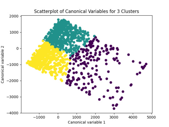
This analysis provides meaningful insights into the underlying structure of attitudes and behaviors in the Outlook on Life Surveys. The three identified clusters represent distinct subgroups of respondents, offering valuable perspectives on how social, political, and cultural factors influence public opinion.

[usesofcannabis]

Generating a Correlation Coefficient

This assignment aims to statistically assess the evidence, provided by NESARC codebook, in favor of or against the association between cannabis use and mental illnesses, such as major depression and general anxiety, in U.S. adults. More specifically, since my research question includes only categorical variables, I selected three new quantitative variables from the NESARC codebook. Therefore, I redefined my hypothesis and examined the correlation between the age when the individuals began using cannabis the most (quantitative explanatory, variable “S3BD5Q2F”) and the age when they experienced the first episode of major depression and general anxiety (quantitative response, variables “S4AQ6A” and ”S9Q6A”). As a result, in the first place, in order to visualize the association between cannabis use and both depression and anxiety episodes, I used seaborn library to produce a scatterplot for each disorder separately and interpreted the overall patterns, by describing the direction, as well as the form and the strength of the relationships. In addition, I ran Pearson correlation test (Q->Q) twice (once for each disorder) and measured the strength of the relationships between each pair of quantitative variables, by numerically generating both the correlation coefficients r and the associated p-values. For the code and the output I used Spyder (IDE).

The three quantitative variables that I used for my Pearson correlation tests are:

  

FOLLWING IS A PYTHON PROGRAM TO CALCULATE CORRELATION

import pandas import numpy import seaborn import scipy import matplotlib.pyplot as plt

nesarc = pandas.read_csv ('nesarc_pds.csv' , low_memory=False)

Set PANDAS to show all columns in DataFrame

pandas.set_option('display.max_columns', None)

Set PANDAS to show all rows in DataFrame

pandas.set_option('display.max_rows', None)

nesarc.columns = map(str.upper , nesarc.columns)

pandas.set_option('display.float_format' , lambda x:'%f'%x)

Change my variables to numeric

nesarc['AGE'] = pandas.to_numeric(nesarc['AGE'], errors='coerce') nesarc['S3BQ4'] = pandas.to_numeric(nesarc['S3BQ4'], errors='coerce') nesarc['S4AQ6A'] = pandas.to_numeric(nesarc['S4AQ6A'], errors='coerce') nesarc['S3BD5Q2F'] = pandas.to_numeric(nesarc['S3BD5Q2F'], errors='coerce') nesarc['S9Q6A'] = pandas.to_numeric(nesarc['S9Q6A'], errors='coerce') nesarc['S4AQ7'] = pandas.to_numeric(nesarc['S4AQ7'], errors='coerce') nesarc['S3BQ1A5'] = pandas.to_numeric(nesarc['S3BQ1A5'], errors='coerce')

Subset my sample

subset1 = nesarc[(nesarc['S3BQ1A5']==1)] # Cannabis users subsetc1 = subset1.copy()

Setting missing data

subsetc1['S3BQ1A5']=subsetc1['S3BQ1A5'].replace(9, numpy.nan) subsetc1['S3BD5Q2F']=subsetc1['S3BD5Q2F'].replace('BL', numpy.nan) subsetc1['S3BD5Q2F']=subsetc1['S3BD5Q2F'].replace(99, numpy.nan) subsetc1['S4AQ6A']=subsetc1['S4AQ6A'].replace('BL', numpy.nan) subsetc1['S4AQ6A']=subsetc1['S4AQ6A'].replace(99, numpy.nan) subsetc1['S9Q6A']=subsetc1['S9Q6A'].replace('BL', numpy.nan) subsetc1['S9Q6A']=subsetc1['S9Q6A'].replace(99, numpy.nan)

Scatterplot for the age when began using cannabis the most and the age of first episode of major depression

plt.figure(figsize=(12,4)) # Change plot size scat1 = seaborn.regplot(x="S3BD5Q2F", y="S4AQ6A", fit_reg=True, data=subset1) plt.xlabel('Age when began using cannabis the most') plt.ylabel('Age when expirenced the first episode of major depression') plt.title('Scatterplot for the age when began using cannabis the most and the age of first the episode of major depression') plt.show()

data_clean=subset1.dropna()

Pearson correlation coefficient for the age when began using cannabis the most and the age of first the episode of major depression

print ('Association between the age when began using cannabis the most and the age of the first episode of major depression') print (scipy.stats.pearsonr(data_clean['S3BD5Q2F'], data_clean['S4AQ6A']))

Scatterplot for the age when began using cannabis the most and the age of the first episode of general anxiety

plt.figure(figsize=(12,4)) # Change plot size scat2 = seaborn.regplot(x="S3BD5Q2F", y="S9Q6A", fit_reg=True, data=subset1) plt.xlabel('Age when began using cannabis the most') plt.ylabel('Age when expirenced the first episode of general anxiety') plt.title('Scatterplot for the age when began using cannabis the most and the age of the first episode of general anxiety') plt.show()

Pearson correlation coefficient for the age when began using cannabis the most and the age of the first episode of general anxiety

print ('Association between the age when began using cannabis the most and the age of first the episode of general anxiety') print (scipy.stats.pearsonr(data_clean['S3BD5Q2F'], data_clean['S9Q6A']))

OUTPUT:

The scatterplot presented above, illustrates the correlation between the age when individuals began using cannabis the most (quantitative explanatory variable) and the age when they experienced the first episode of depression (quantitative response variable). The direction of the relationship is positive (increasing), which means that an increase in the age of cannabis use is associated with an increase in the age of the first depression episode. In addition, since the points are scattered about a line, the relationship is linear. Regarding the strength of the relationship, from the pearson correlation test we can see that the correlation coefficient is equal to 0.23, which indicates a weak linear relationship between the two quantitative variables. The associated p-value is equal to 2.27e-09 (p-value is written in scientific notation) and the fact that its is very small means that the relationship is statistically significant. As a result, the association between the age when began using cannabis the most and the age of the first depression episode is moderately weak, but it is highly unlikely that a relationship of this magnitude would be due to chance alone. Finally, by squaring the r, we can find the fraction of the variability of one variable that can be predicted by the other, which is fairly low at 0.05.

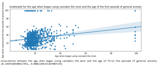
For the association between the age when individuals began using cannabis the most (quantitative explanatory variable) and the age when they experienced the first episode of anxiety (quantitative response variable), the scatterplot psented above shows a positive linear relationship. Regarding the strength of the relationship, the pearson correlation test indicates that the correlation coefficient is equal to 0.14, which is interpreted to a fairly weak linear relationship between the two quantitative variables. The associated p-value is equal to 0.0001, which means that the relationship is statistically significant. Therefore, the association between the age when began using cannabis the most and the age of the first anxiety episode is weak, but it is highly unlikely that a relationship of this magnitude would be due to chance alone. Finally, by squaring the r, we can find the fraction of the variability of one variable that can be predicted by the other, which is very low at 0.01.

[konio011]

Running a Classification Tree

Code:

import pandas as pd import os from sklearn.model_selection import train_test_split from sklearn.tree import DecisionTreeClassifier import sklearn.metrics

AH_data = pd.read_csv("tree_addhealth.csv")

data_clean = AH_data.dropna()

data_clean.dtypes data_clean.describe()

predictors = data_clean[['BIO_SEX','WHITE','BLACK','ASIAN','age']]

targets = data_clean.TREG1

pred_train, pred_test, tar_train, tar_test = train_test_split(predictors, targets, test_size=.4)

pred_train.shape pred_test.shape tar_train.shape tar_test.shape

classifier=DecisionTreeClassifier(max_leaf_nodes=8) classifier=classifier.fit(pred_train,tar_train)

predictions=classifier.predict(pred_test)

sklearn.metrics.confusion_matrix(tar_test,predictions) sklearn.metrics.accuracy_score(tar_test, predictions)

from sklearn import tree

from io import StringIO

from StringIO import StringIO

from IPython.display import Image out = StringIO() tree.export_graphviz(classifier, out_file=out) import pydotplus graph=pydotplus.graph_from_dot_data(out.getvalue()) Image(graph.create_png())

Decission Tree:

Interpretation:

Decision tree analysis was done for classification problem related smoking problem (evaluation base on BIO_SEX,Color (White/Black), Nation (Asian) and age features).

The first variable to separate was color (white). White people were non-regular smokers than black ones.

Most of white, young people below around 17-18 years were non-regular smokers, but 212 of them were regular smokers. In comparison for black ones: most of teenagers below 15-16 were regular smokers, but there was quite narrow margin.

In black people we observed we observed similar number of smokers and non-regular smokers in relation to gender, but for male above 18 years old manly there were regular smokers.

[introduccionalanalisisdedatos]

#Convertir variables a numérico

data['PPAGECAT'] = pandas.to_numeric(data['PPAGECAT'], errors='coerce') data['W1_C1'] = pandas.to_numeric(data['W1_C1'], errors='coerce') data['PPEDUC'] = pandas.to_numeric(data['PPEDUC'], errors='coerce')

#Eliminar filas con valores NaN

data_clean = data.dropna(subset=['PPAGECAT', 'W1_C1', 'PPEDUC'])

#Crear grupos basados en niveles de educación

educ_groups = data_clean['PPEDUC'].unique()

#Calcular la correlación de Pearson dentro de cada grupo

for group in educ_groups: subset = data_clean[data_clean['PPEDUC'] == group] if len(subset) < 2: print(f"Nivel de Educación {group}: No hay suficientes datos para calcular la correlación (n < 2).") continuepearson_corr, p_value = pearsonr(subset['PPAGECAT'], subset['W1_C1']) print(f"Nivel de Educación {group}:") print(f"Coeficiente de correlación de Pearson: {pearson_corr}") print(f"Valor p: {p_value}") print(f"Coeficiente de Determinación (R^2): {pearson_corr**2}") print()

Los resultados de la prueba Chi-cuadrado indican que no existe una asociación significativa entre las categorías de edad y la afiliación política (p = 0.1857). Esto sugiere que la edad no es un factor determinante en la afiliación política de los encuestados.

En cuanto a la correlación de Pearson moderada por el nivel de educación, encontramos que la mayoría de las correlaciones no son significativas. Solo el grupo con nivel de educación 9 mostró una correlación significativa, aunque débil (Pearson r = -0.0778, p = 0.0397). Esto sugiere que, en general, el nivel de educación no modera fuertemente la relación entre la edad y la afiliación política.

Este análisis muestra la importancia de considerar factores moderadores al estudiar relaciones entre variables. Aunque no se encontró una fuerte moderación en este caso, es posible que otros factores podrían revelar asociaciones significativas.

[intelarti]

RandomForest Project

from pandas import Series, DataFrame import pandas as pd import numpy as np import os import matplotlib.pylab as plt from sklearn.model_selection import train_test_split from sklearn.tree import DecisionTreeClassifier from sklearn.metrics import classification_report import sklearn.metrics

# Feature Importance from sklearn import datasets from sklearn.ensemble import ExtraTreesClassifier

""" Modeling and Prediction

Split into training and testing sets """

predictors = data_clean[[ 'CODPRIPER', 'CODULTPER', 'SEXOC']]

targets = data_clean.SITALUC

pred_train, pred_test, tar_train, tar_test = train_test_split(predictors, targets, test_size=.4)

pred_train.shape pred_test.shape tar_train.shape tar_test.shape

#Build model on training data

from sklearn.ensemble import RandomForestClassifier

classifier=RandomForestClassifier(n_estimators=25) classifier=classifier.fit(pred_train,tar_train)

predictions=classifier.predict(pred_test)

sklearn.metrics.confusion_matrix(tar_test,predictions) sklearn.metrics.accuracy_score(tar_test, predictions)

""" Running a different number of trees and see the effect of that on the accuracy of the prediction """

trees=range(25) accuracy=np.zeros(25)

for idx in range(len(trees)): classifier=RandomForestClassifier(n_estimators=idx + 1) classifier=classifier.fit(pred_train,tar_train) predictions=classifier.predict(pred_test) accuracy[idx]=sklearn.metrics.accuracy_score(tar_test, predictions)

plt.cla() plt.plot(trees, accuracy)

The accuracy of a RandomForestClassifier varies with the number of trees (n_estimators). A RandomForestClassifier is trained and evaluated with an increasing number of trees, from 1 up to the size of the trees list. The resulting accuracy for each number of trees is plotted, allowing visualization of the impact of the number of trees on the model's accuracy, that is growing.

This type of analysis is useful for determining the optimal number of trees in a random forest, balancing the improvement in accuracy with the additional computational cost of adding more trees.

[mengchunhsieh]

K-means clusthering

#importamos las librerías necesarias

from pandas import Series,DataFrame

import pandas as pd

import numpy as np

import matplotlib.pylab as plt

from sklearn.model_selection

import train_test_splitfrom sklearn

import preprocessing

from sklearn.cluster import KMeans

"""Data Management"""

data =pd.read_csv("/content/drive/MyDrive/tree_addhealth.csv" )

#upper-case all DataFrame column names

data.columns = map(str.upper, data.columns)

# Data Managementdata_clean = data.dropna()

# subset clustering variablescluster=data_clean[['ALCEVR1','MAREVER1','ALCPROBS1','DEVIANT1','VIOL1','DEP1','ESTEEM1','SCHCONN1','PARACTV', 'PARPRES','FAMCONCT']]

cluster.describe()

# standardize clustering variables to have mean=0 and sd=1

clustervar=cluster.copy()

clustervar['ALCEVR1']=preprocessing.scale(clustervar['ALCEVR1'].astype('float64'))

clustervar['ALCPROBS1']=preprocessing.scale(clustervar['ALCPROBS1'].astype('float64'))

clustervar['MAREVER1']=preprocessing.scale(clustervar['MAREVER1'].astype('float64'))

clustervar['DEP1']=preprocessing.scale(clustervar['DEP1'].astype('float64'))

clustervar['ESTEEM1']=preprocessing.scale(clustervar['ESTEEM1'].astype('float64'))

clustervar['VIOL1']=preprocessing.scale(clustervar['VIOL1'].astype('float64'))

clustervar['DEVIANT1']=preprocessing.scale(clustervar['DEVIANT1'].astype('float64'))

clustervar['FAMCONCT']=preprocessing.scale(clustervar['FAMCONCT'].astype('float64'))

clustervar['SCHCONN1']=preprocessing.scale(clustervar['SCHCONN1'].astype('float64'))

clustervar['PARACTV']=preprocessing.scale(clustervar['PARACTV'].astype('float64'))

clustervar['PARPRES']=preprocessing.scale(clustervar['PARPRES'].astype('float64'))

# split data into train and test sets

clus_train, clus_test = train_test_split(clustervar, test_size=.3, random_state=123)

# k-means cluster analysis for 1-9 clusters

from scipy.spatial.distance import cdist

clusters=range(1,10)

meandist=[]

for k in clusters: model=KMeans(n_clusters=k) model.fit(clus_train) clusassign=model.predict(clus_train) meandist.append(sum(np.min(cdist(clus_train, model.cluster_centers_, 'euclidean'), axis=1))

/ clus_train.shape[0])

"""Plot average distance from observations from the cluster centroidto use the Elbow Method to identify number of clusters to choose"""

plt.plot(clusters,meandist)

plt.xlabel('Number of clusters')

plt.ylabel('Average distance')

plt.title('Selecting k with the Elbow Method')

# Interpret 2 cluster solution

model2=KMeans(n_clusters=2)model2.fit(clus_train)

clusassign=model2.predict(clus_train)

# plot clusters

from sklearn.decomposition import PCA

pca_2 = PCA(2)

plot_columns = pca_2.fit_transform(clus_train)

plt.scatter(x=plot_columns[:,0],y=plot_columns[:,1],c=model2.labels_,)

plt.xlabel('Canonical variable 1')

plt.ylabel('Canonical variable 2')

plt.title('Scatterplot of Canonical Variables for 2 Clusters')

plt.show()

"""BEGIN multiple steps to merge cluster assignment with clustering variables to examinecluster variable means by cluster"""

# create a unique identifier variable from the index for the

# cluster training data to merge with the cluster assignment variable

clus_train.reset_index(level=0, inplace=True)

# create a list that has the new index variable

cluslist=list(clus_train['index'])

# create a list of cluster assignments

labels=list(model2.labels_)

# combine index variable list with cluster assignment list into a dictionary

newlist=dict(zip(cluslist, labels))newlist

# convert newlist dictionary to a dataframenew

clus=DataFrame.from_dict(newlist, orient='index')newclus

# rename the cluster assignment columnnew

clus.columns = ['cluster']

# now do the same for the cluster assignment variable

# create a unique identifier variable from the index for the

# cluster assignment dataframe

# to merge with cluster training datanew

clus.reset_index(level=0, inplace=True)

# merge the cluster assignment dataframe with the cluster training variable dataframe

# by the index variablemerged_train=pd.merge(clus_train, newclus, on='index')

merged_train.head(n=100)

# cluster frequenciesmerged_train.cluster.value_counts()

"""END multiple steps to merge cluster assignment with clustering variables to examinecluster variable means by cluster"""

# FINALLY calculate clustering variable means by

clusterclustergrp = merged_train.groupby('cluster').mean()print ("Clustering variable means by cluster")

print(clustergrp)

# validate clusters in training data by examining cluster differences in GPA using ANOVA

# first have to merge GPA with clustering variables and cluster assignment data

gpa_data=data_clean['GPA1']

# split GPA data into train and test sets

gpa_train, gpa_test = train_test_split(gpa_data, test_size=.3, random_state=123)

gpa_train1=pd.DataFrame(gpa_train)

gpa_train1.reset_index(level=0, inplace=True)

merged_train_all=pd.merge(gpa_train1, merged_train, on='index')

sub1 = merged_train_all[['GPA1', 'cluster']].dropna()

import statsmodels.formula.api as smf

import statsmodels.stats.multicomp as multi

gpamod = smf.ols(formula='GPA1 ~ C(cluster)', data=sub1).fit()

print (gpamod.summary())

print ('means for GPA by cluster')

m1= sub1.groupby('cluster').mean()

print (m1)

print ('standard deviations for GPA by cluster')

m2= sub1.groupby('cluster').std()print (m2)

mc1 = multi.MultiComparison(sub1['GPA1'], sub1['cluster'])

res1 = mc1.tukeyhsd()

print(res1.summary())

爆發

0 則迴響

[rogerscode]

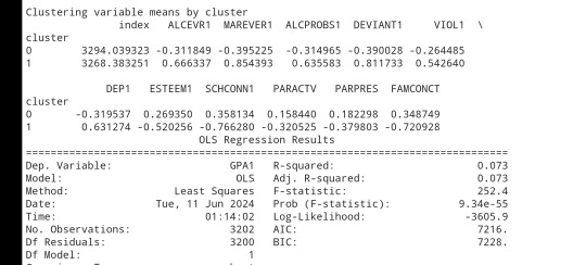
K-means clusthering

#importamos las librerías necesarias

from pandas import Series,DataFrame

import pandas as pd

import numpy as np

import matplotlib.pylab as plt

from sklearn.model_selection

import train_test_splitfrom sklearn

import preprocessing

from sklearn.cluster import KMeans

"""Data Management"""

data =pd.read_csv("/content/drive/MyDrive/tree_addhealth.csv" )

#upper-case all DataFrame column names

data.columns = map(str.upper, data.columns)

# Data Managementdata_clean = data.dropna()

# subset clustering variablescluster=data_clean[['ALCEVR1','MAREVER1','ALCPROBS1','DEVIANT1','VIOL1','DEP1','ESTEEM1','SCHCONN1','PARACTV', 'PARPRES','FAMCONCT']]

cluster.describe()

# standardize clustering variables to have mean=0 and sd=1

clustervar=cluster.copy()

clustervar['ALCEVR1']=preprocessing.scale(clustervar['ALCEVR1'].astype('float64'))

clustervar['ALCPROBS1']=preprocessing.scale(clustervar['ALCPROBS1'].astype('float64'))

clustervar['MAREVER1']=preprocessing.scale(clustervar['MAREVER1'].astype('float64'))

clustervar['DEP1']=preprocessing.scale(clustervar['DEP1'].astype('float64'))

clustervar['ESTEEM1']=preprocessing.scale(clustervar['ESTEEM1'].astype('float64'))

clustervar['VIOL1']=preprocessing.scale(clustervar['VIOL1'].astype('float64'))

clustervar['DEVIANT1']=preprocessing.scale(clustervar['DEVIANT1'].astype('float64'))

clustervar['FAMCONCT']=preprocessing.scale(clustervar['FAMCONCT'].astype('float64'))

clustervar['SCHCONN1']=preprocessing.scale(clustervar['SCHCONN1'].astype('float64'))

clustervar['PARACTV']=preprocessing.scale(clustervar['PARACTV'].astype('float64'))

clustervar['PARPRES']=preprocessing.scale(clustervar['PARPRES'].astype('float64'))

# split data into train and test sets

clus_train, clus_test = train_test_split(clustervar, test_size=.3, random_state=123)

# k-means cluster analysis for 1-9 clusters

from scipy.spatial.distance import cdist

clusters=range(1,10)

meandist=[]

for k in clusters: model=KMeans(n_clusters=k) model.fit(clus_train) clusassign=model.predict(clus_train) meandist.append(sum(np.min(cdist(clus_train, model.cluster_centers_, 'euclidean'), axis=1))

/ clus_train.shape[0])

"""Plot average distance from observations from the cluster centroidto use the Elbow Method to identify number of clusters to choose"""

plt.plot(clusters,meandist)

plt.xlabel('Number of clusters')

plt.ylabel('Average distance')

plt.title('Selecting k with the Elbow Method')

# Interpret 2 cluster solution

model2=KMeans(n_clusters=2)model2.fit(clus_train)

clusassign=model2.predict(clus_train)

# plot clusters

from sklearn.decomposition import PCA

pca_2 = PCA(2)

plot_columns = pca_2.fit_transform(clus_train)

plt.scatter(x=plot_columns[:,0],y=plot_columns[:,1],c=model2.labels_,)

plt.xlabel('Canonical variable 1')

plt.ylabel('Canonical variable 2')

plt.title('Scatterplot of Canonical Variables for 2 Clusters')

plt.show()

"""BEGIN multiple steps to merge cluster assignment with clustering variables to examinecluster variable means by cluster"""

# create a unique identifier variable from the index for the

# cluster training data to merge with the cluster assignment variable

clus_train.reset_index(level=0, inplace=True)

# create a list that has the new index variable

cluslist=list(clus_train['index'])

# create a list of cluster assignments

labels=list(model2.labels_)

# combine index variable list with cluster assignment list into a dictionary

newlist=dict(zip(cluslist, labels))newlist

# convert newlist dictionary to a dataframenew

clus=DataFrame.from_dict(newlist, orient='index')newclus

# rename the cluster assignment columnnew

clus.columns = ['cluster']

# now do the same for the cluster assignment variable

# create a unique identifier variable from the index for the

# cluster assignment dataframe

# to merge with cluster training datanew

clus.reset_index(level=0, inplace=True)

# merge the cluster assignment dataframe with the cluster training variable dataframe

# by the index variablemerged_train=pd.merge(clus_train, newclus, on='index')

merged_train.head(n=100)

# cluster frequenciesmerged_train.cluster.value_counts()

"""END multiple steps to merge cluster assignment with clustering variables to examinecluster variable means by cluster"""

# FINALLY calculate clustering variable means by

clusterclustergrp = merged_train.groupby('cluster').mean()print ("Clustering variable means by cluster")

print(clustergrp)

# validate clusters in training data by examining cluster differences in GPA using ANOVA

# first have to merge GPA with clustering variables and cluster assignment data

gpa_data=data_clean['GPA1']

# split GPA data into train and test sets

gpa_train, gpa_test = train_test_split(gpa_data, test_size=.3, random_state=123)

gpa_train1=pd.DataFrame(gpa_train)

gpa_train1.reset_index(level=0, inplace=True)

merged_train_all=pd.merge(gpa_train1, merged_train, on='index')

sub1 = merged_train_all[['GPA1', 'cluster']].dropna()

import statsmodels.formula.api as smf

import statsmodels.stats.multicomp as multi

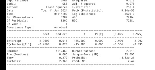
gpamod = smf.ols(formula='GPA1 ~ C(cluster)', data=sub1).fit()

print (gpamod.summary())

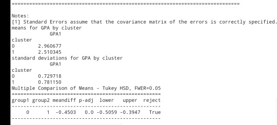
print ('means for GPA by cluster')

m1= sub1.groupby('cluster').mean()

print (m1)

print ('standard deviations for GPA by cluster')

m2= sub1.groupby('cluster').std()print (m2)

mc1 = multi.MultiComparison(sub1['GPA1'], sub1['cluster'])

res1 = mc1.tukeyhsd()

print(res1.summary())

[123bhaawna]

Running a Random Forecast

from pandas import Series, DataFrame import pandas as pd import numpy as np import os import matplotlib.pylab as plt from sklearn.cross_validation import train_test_split from sklearn.tree import DecisionTreeClassifier from sklearn.metrics import classification_report import sklearn.metrics # Feature Importance from sklearn import datasets from sklearn.ensemble import ExtraTreesClassifier

os.chdir("C:\Users\ASUS\Downloads")

Load the dataset

AH_data = pd.read_csv("tree_addhealth.csv") data_clean = AH_data.dropna()

data_clean.dtypes data_clean.describe()

Split into training and testing sets

predictors = data_clean[['BIO_SEX','HISPANIC','WHITE','BLACK','NAMERICAN','ASIAN','age', 'ALCEVR1','ALCPROBS1','marever1','cocever1','inhever1','cigavail','DEP1','ESTEEM1','VIOL1', 'PASSIST','DEVIANT1','SCHCONN1','GPA1','EXPEL1','FAMCONCT','PARACTV','PARPRES']]

targets = data_clean.TREG1

pred_train, pred_test, tar_train, tar_test = train_test_split(predictors, targets, test_size=.4)

pred_train.shape pred_test.shape tar_train.shape tar_test.shape

Build model on training data

from sklearn.ensemble import RandomForestClassifier

classifier=RandomForestClassifier(n_estimators=25) classifier=classifier.fit(pred_train,tar_train)

predictions=classifier.predict(pred_test)

sklearn.metrics.confusion_matrix(tar_test,predictions) sklearn.metrics.accuracy_score(tar_test, predictions)

fit an Extra Trees model to the data

model = ExtraTreesClassifier() model.fit(pred_train,tar_train)

display the relative importance of each attribute

print(model.feature_importances_)

""" Running a different number of trees and see the effect of that on the accuracy of the prediction """

trees=range(25) accuracy=np.zeros(25)

for idx in range(len(trees)): classifier=RandomForestClassifier(n_estimators=idx + 1) classifier=classifier.fit(pred_train,tar_train) predictions=classifier.predict(pred_test) accuracy[idx]=sklearn.metrics.accuracy_score(tar_test, predictions)

plt.cla() plt.plot(trees, accuracy)

OUTPUT:

[0.02674519 0.01452508 0.02383281 0.01552068 0.00653599 0.00626536 0.06307556 0.05160827 0.04981202 0.10180787 0.01907461 0.01705372 0.02688986 0.05987085 0.05729702 0.04918319 0.01754836 0.07740653 0.06704035 0.07006239 0.01263347 0.05856173 0.05589433 0.05175476]

The most correlated variable is marijuana use, while the smallest correlation is obtained from being American.

The accuracy mostly goes up to 85%. Thus, a limited number of trees with slightly lower accuracy, 83%, is enough for this model.

[viianey-gutma]

Data Analysis Tools - Correlation

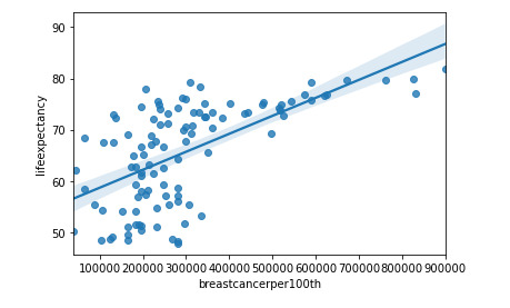
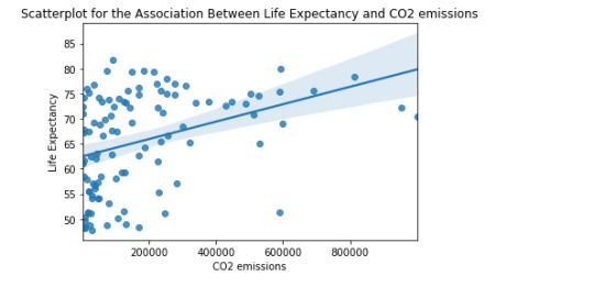
The objective is to generate a Correlation Coefficient, this type of coefficient is used when there are two quantitative variables. For this task, the correlation between life expectancy, CO2 emissions and breast cancer will be used. The dataset used is gap Minder (https://www.gapminder.org/).

Python code

import pandas as pd import numpy import seaborn import scipy import matplotlib.pyplot as plt

df = pd.read_csv('gapminder.csv', low_memory=False)

df['co2emissions'] = df['co2emissions'].apply(pd.to_numeric, errors='coerce') df['breastcancerper100th'] = df['breastcancerper100th'].apply(pd.to_numeric, errors='coerce') df['lifeexpectancy'] = df['lifeexpectancy'].apply(pd.to_numeric, errors='coerce')

df=df[(df['lifeexpectancy']>=1) & (df['lifeexpectancy']<=100) & (df['co2emissions']<1000000000) ]

print(max(df['co2emissions'])) print(min(df['co2emissions']))

df['lifeexpectancy']=df['lifeexpectancy'].replace(' ', numpy.nan) df['co2emissions']=df['co2emissions'].replace(' ', numpy.nan) df['breastcancerper100th']=df['breastcancerper100th'].replace(' ', numpy.nan)

df.breastcancerper100th *=10000 df.co2emissions /=1000

df1=df.dropna() df2=df1

graf1= seaborn.regplot(x="breastcancerper100th", y="lifeexpectancy", fit_reg=True, data=df1)

plt.xlabel('Breast cancer') plt.ylabel('Life Expectancy') plt.title('Scatterplot for the Association Between Life Expectancy and Breast cancer')

graf2 = seaborn.regplot(x="co2emissions", y="lifeexpectancy", fit_reg=True, data=df1) plt.xlabel('CO2 emissions') plt.ylabel('Life Expectancy') plt.title('Scatterplot for the Association Between Life Expectancy and CO2 emissions') data_clean=df.dropna()

print ('association between Life Expectancy and co2emissions') print (scipy.stats.pearsonr(data_clean['co2emissions'], data_clean['lifeexpectancy']))

print ('association between Life Expectancy and Breast cancer') print (scipy.stats.pearsonr(data_clean['breastcancerper100th'], data_clean['lifeexpectancy']))

[edujournalblogs]

Data Science is the field of finding out solutions to a particular problem by analyzing the data that are fact-based and real-time in nature. For instance, suppose a company is facing problem with its sales or marketing or profit margin is shrinking etc. In such a scenario, the company will reach out to a data scientist who will execute a particular process. The process could be in the form of :

Identification the data analytical problem ie whether the fluctuation is due to pricing not set right, or specific marketing fluctuation which is constant for all other products or is it specific to this organization alone. So all these are analyzed and the data scientist will find out the actual underlined problem.

Gather all the information related to the problem in hand.

Dataset could be in a structured or unstructured form. Structured form could mean a file in a tabular form such as excel, mysql, sql server etc. Unstructured form could mean images, videos, audio, social media site etc.

Data collected from various sources must be cleaned and validated to ensure accuracy, completeness and uniformity.

Try to find out what model that fits the best for the given problem. The dataset is aligned to a particular model and algorithm is applied to this data, and the data is analyzed and different trends and patterns are extracted out of it.

Once patterns and trends are found out, the interpretation of data to discover solutions and opportunities is done for our company and find different solutions.

Communicate these findings to stakeholders using visualization for better understanding.

Check out our master program in Data Science and ASP.NET- Complete Beginner to Advanced course and boost your confidence and knowledge.

URL: www.edujournal.com

[machinelearner01]

from pandas import Series, DataFrame import pandas as pd import numpy as np import os import matplotlib.pylab as plt from sklearn.cross_validation import train_test_split from sklearn.tree import DecisionTreeClassifier from sklearn.metrics import classification_report import sklearn.metrics # Feature Importance from sklearn import datasets from sklearn.ensemble import ExtraTreesClassifier

os.chdir("C:\Users\ASUS\Downloads")

Load the dataset

AH_data = pd.read_csv("tree_addhealth.csv") data_clean = AH_data.dropna()

data_clean.dtypes data_clean.describe()

Split into training and testing sets

predictors = data_clean[['BIO_SEX','HISPANIC','WHITE','BLACK','NAMERICAN','ASIAN','age', 'ALCEVR1','ALCPROBS1','marever1','cocever1','inhever1','cigavail','DEP1','ESTEEM1','VIOL1', 'PASSIST','DEVIANT1','SCHCONN1','GPA1','EXPEL1','FAMCONCT','PARACTV','PARPRES']]

targets = data_clean.TREG1

pred_train, pred_test, tar_train, tar_test = train_test_split(predictors, targets, test_size=.4)

pred_train.shape pred_test.shape tar_train.shape tar_test.shape

Build model on training data

from sklearn.ensemble import RandomForestClassifier

classifier=RandomForestClassifier(n_estimators=25) classifier=classifier.fit(pred_train,tar_train)

predictions=classifier.predict(pred_test)

sklearn.metrics.confusion_matrix(tar_test,predictions) sklearn.metrics.accuracy_score(tar_test, predictions)

fit an Extra Trees model to the data

model = ExtraTreesClassifier() model.fit(pred_train,tar_train)

display the relative importance of each attribute

print(model.feature_importances_)

""" Running a different number of trees and see the effect of that on the accuracy of the prediction """

trees=range(25) accuracy=np.zeros(25)

for idx in range(len(trees)): classifier=RandomForestClassifier(n_estimators=idx + 1) classifier=classifier.fit(pred_train,tar_train) predictions=classifier.predict(pred_test) accuracy[idx]=sklearn.metrics.accuracy_score(tar_test, predictions)

plt.cla() plt.plot(trees, accuracy)

OUTPUT:

[0.02674519 0.01452508 0.02383281 0.01552068 0.00653599 0.00626536 0.06307556 0.05160827 0.04981202 0.10180787 0.01907461 0.01705372 0.02688986 0.05987085 0.05729702 0.04918319 0.01754836 0.07740653 0.06704035 0.07006239 0.01263347 0.05856173 0.05589433 0.05175476]

The most correlated variable is marijuana use, while the smallest correlation is obtained from being American.

The accuracy mostly goes up to 85%. Thus, a limited number of trees with slightly lower accuracy, 83%, is enough for this model.

[pinguinportfoli0]

OOL Attacker - Running a Lasso Regression Analysis

For this project it was used the Outlook on Life Surveys. "The purpose of the 2012 Outlook Surveys were to study political and social attitudes in the United States. The specific purpose of the survey is to consider the ways in which social class, ethnicity, marital status, feminism, religiosity, political orientation, and cultural beliefs or stereotypes influence opinion and behavior." - Outlook

Was necessary the removal of some rows containing text (for confidentiality purposes) before the dorpna() function.

This is my full code:

import pandas as pd import numpy as np import matplotlib.pylab as plt from sklearn.model_selection import train_test_split from sklearn.linear_model import LassoLarsCV from sklearn import preprocessing import time #Load the dataset data = pd.read_csv(r"PATHHHH") #upper-case all DataFrame column names data.columns = map(str.upper, data.columns) # Data Management data_clean = data.select_dtypes(include=['number']) data_clean = data_clean.dropna() print(data_clean.describe()) print(data_clean.dtypes) #Split into training and testing sets headers = list(data_clean.columns) headers.remove("PPNET") predvar = data_clean[headers] target = data_clean.PPNET predictors=predvar.copy() for header in headers:     predictors[header] = preprocessing.scale(predictors[header].astype('float64')) # split data into train and test sets pred_train, pred_test, tar_train, tar_test = train_test_split(predictors, target, test_size=.3, random_state=123) # specify the lasso regression model model=LassoLarsCV(cv=10, precompute=False).fit(pred_train,tar_train) #Display both categories by coefs pd.set_option('display.max_rows', None) table_catimp=pd.DataFrame({'cat': predictors.columns, 'coef': abs(model.coef_)}) print(table_catimp) non_zero_count = (table_catimp['coef'] != 0).sum() zero_count = table_catimp.shape[0] - non_zero_count print(f"Number of non-zero coefficients: {non_zero_count}") print(f"Number of zero coefficients: {zero_count}") #Display top 5 categories by coefs top_5_rows = table_catimp.nlargest(10, 'coef') print(top_5_rows.to_string(index=False)) # plot coefficient progression m_log_alphas = -np.log10(model.alphas_) ax = plt.gca() plt.plot(m_log_alphas, model.coef_path_.T) plt.axvline(-np.log10(model.alpha_), linestyle='--', color='k',             label='alpha CV') plt.ylabel('Regression Coefficients') plt.xlabel('-log(alpha)') plt.title('Regression Coefficients Progression for Lasso Paths') # plot mean square error for each fold m_log_alphascv = -np.log10(model.cv_alphas_) plt.figure() plt.plot(m_log_alphascv, model.mse_path_, ':') plt.plot(m_log_alphascv, model.mse_path_.mean(axis=-1), 'k',          label='Average across the folds', linewidth=2) plt.axvline(-np.log10(model.alpha_), linestyle='--', color='k',             label='alpha CV') plt.legend() plt.xlabel('-log(alpha)') plt.ylabel('Mean squared error') plt.title('Mean squared error on each fold') # MSE from training and test data from sklearn.metrics import mean_squared_error train_error = mean_squared_error(tar_train, model.predict(pred_train)) test_error = mean_squared_error(tar_test, model.predict(pred_test)) print ('training data MSE') print(train_error) print ('test data MSE') print(test_error) # R-square from training and test data rsquared_train=model.score(pred_train,tar_train) rsquared_test=model.score(pred_test,tar_test) print ('training data R-square') print(rsquared_train) print ('test data R-square') print(rsquared_test) plt.show()

Output:

Number of non-zero coefficients: 54 Number of zero coefficients: 186 training data MSE: 0.11867468892072082 test data MSE: 0.1458371486851879 training data R-square: 0.29967753231880834 test data R-square: 0.18204209521525183

Top 10 coefs:

PPINCIMP 0.097772 W1_WEIGHT3 0.061791 W1_P21 0.048740 W1_E1 0.027003 W1_CASEID 0.026709 PPHHSIZE 0.026055 PPAGECT4 0.022809 W1_Q1_B 0.021630 W1_P16E 0.020672 W1_E63_C 0.020205

Conclusions:

While the test error is slightly higher than the training error, the difference is not extreme, which is a positive sign that the model generalizes reasonably well.

Also in another note, the drop in R-square between training and test sets suggests the model may be overfitting slightly or that the predictors do not fully explain the response variable's behavior.

In the attachments I present the Regression coefficients, allowing to verify which features or characteristics are the most relevant for this model. Both PPINCIMP and W1_WEIGHT3 have the biggest weight. In the second attachment we can select the optimal alpha, the vertical dashed line indicates the optimal value of alpha.

The program successfully identified a subset of 54 predictors from 240 variables that are most strongly associated with the response variable. The moderate R-square values suggest room for improvement in the model's explanatory power. However, the close alignment between training and test MSE indicates reasonable generalization.

[machine-learning-coursera]

Machine Learning for Data Analysis

Week 4: Running a k-means Cluster Analysis

A k-means cluster analysis was conducted to identify underlying subgroups of countries based on their similarity of responses on 7 variables that represent characteristics that could have an impact on internet use rates. Clustering variables included quantitative variables measuring income per person, employment rate, female employment rate, polity score, alcohol consumption, life expectancy, and urban rate. All clustering variables were standardized to have a mean of 0 and a standard deviation of 1.

Because the GapMinder dataset which I am using is relatively small (N < 250), I have not split the data into test and training sets. A series of k-means cluster analyses were conducted on the training data specifying k=1-9 clusters, using Euclidean distance. The variance in the clustering variables that was accounted for by the clusters (r-square) was plotted for each of the nine cluster solutions in an elbow curve to provide guidance for choosing the number of clusters to interpret.

Load the data, set the variables to numeric, and clean the data of NA values

In [1]:import pandas as pd import numpy as np import matplotlib.pyplot as plt import statsmodels.formula.api as smf import statsmodels.stats.multicomp as multi from sklearn.cross_validation import train_test_split from sklearn import preprocessing from sklearn.cluster import KMeans data = pd.read_csv('c:/users/greg/desktop/gapminder.csv', low_memory=False) data['internetuserate'] = pd.to_numeric(data['internetuserate'], errors='coerce') data['incomeperperson'] = pd.to_numeric(data['incomeperperson'], errors='coerce') data['employrate'] = pd.to_numeric(data['employrate'], errors='coerce') data['femaleemployrate'] = pd.to_numeric(data['femaleemployrate'], errors='coerce') data['polityscore'] = pd.to_numeric(data['polityscore'], errors='coerce') data['alcconsumption'] = pd.to_numeric(data['alcconsumption'], errors='coerce') data['lifeexpectancy'] = pd.to_numeric(data['lifeexpectancy'], errors='coerce') data['urbanrate'] = pd.to_numeric(data['urbanrate'], errors='coerce') sub1 = data.copy() data_clean = sub1.dropna()

Subset the clustering variables

In [2]:cluster = data_clean[['incomeperperson','employrate','femaleemployrate','polityscore', 'alcconsumption', 'lifeexpectancy', 'urbanrate']] cluster.describe()

Out[2]:incomeperpersonemployratefemaleemployratepolityscorealcconsumptionlifeexpectancyurbanratecount150.000000150.000000150.000000150.000000150.000000150.000000150.000000mean6790.69585859.26133348.1006673.8933336.82173368.98198755.073200std9861.86832710.38046514.7809996.2489165.1219119.90879622.558074min103.77585734.90000212.400000-10.0000000.05000048.13200010.40000025%592.26959252.19999939.599998-1.7500002.56250062.46750036.41500050%2231.33485558.90000248.5499997.0000006.00000072.55850057.23000075%7222.63772165.00000055.7250009.00000010.05750076.06975071.565000max39972.35276883.19999783.30000310.00000023.01000083.394000100.000000

Standardize the clustering variables to have mean = 0 and standard deviation = 1

In [3]:clustervar=cluster.copy() clustervar['incomeperperson']=preprocessing.scale(clustervar['incomeperperson'].astype('float64')) clustervar['employrate']=preprocessing.scale(clustervar['employrate'].astype('float64')) clustervar['femaleemployrate']=preprocessing.scale(clustervar['femaleemployrate'].astype('float64')) clustervar['polityscore']=preprocessing.scale(clustervar['polityscore'].astype('float64')) clustervar['alcconsumption']=preprocessing.scale(clustervar['alcconsumption'].astype('float64')) clustervar['lifeexpectancy']=preprocessing.scale(clustervar['lifeexpectancy'].astype('float64')) clustervar['urbanrate']=preprocessing.scale(clustervar['urbanrate'].astype('float64'))

Split the data into train and test sets

In [4]:clus_train, clus_test = train_test_split(clustervar, test_size=.3, random_state=123)

Perform k-means cluster analysis for 1-9 clusters

In [5]:from scipy.spatial.distance import cdist clusters = range(1,10) meandist = [] for k in clusters: model = KMeans(n_clusters = k) model.fit(clus_train) clusassign = model.predict(clus_train) meandist.append(sum(np.min(cdist(clus_train, model.cluster_centers_, 'euclidean'), axis=1)) / clus_train.shape[0])

Plot average distance from observations from the cluster centroid to use the Elbow Method to identify number of clusters to choose

In [6]:plt.plot(clusters, meandist) plt.xlabel('Number of clusters') plt.ylabel('Average distance') plt.title('Selecting k with the Elbow Method') plt.show()

Interpret 3 cluster solution

In [7]:model3 = KMeans(n_clusters=4) model3.fit(clus_train) clusassign = model3.predict(clus_train)

Plot the clusters

In [8]:from sklearn.decomposition import PCA pca_2 = PCA(2) plt.figure() plot_columns = pca_2.fit_transform(clus_train) plt.scatter(x=plot_columns[:,0], y=plot_columns[:,1], c=model3.labels_,) plt.xlabel('Canonical variable 1') plt.ylabel('Canonical variable 2') plt.title('Scatterplot of Canonical Variables for 4 Clusters') plt.show()

Begin multiple steps to merge cluster assignment with clustering variables to examine cluster variable means by cluster.

Create a unique identifier variable from the index for the cluster training data to merge with the cluster assignment variable.

In [9]:clus_train.reset_index(level=0, inplace=True)

Create a list that has the new index variable

In [10]:cluslist = list(clus_train['index'])

Create a list of cluster assignments

In [11]:labels = list(model3.labels_)

Combine index variable list with cluster assignment list into a dictionary

In [12]:newlist = dict(zip(cluslist, labels)) print (newlist) {2: 1, 4: 2, 6: 0, 10: 0, 11: 3, 14: 2, 16: 3, 17: 0, 19: 2, 22: 2, 24: 3, 27: 3, 28: 2, 29: 2, 31: 2, 32: 0, 35: 2, 37: 3, 38: 2, 39: 3, 42: 2, 45: 2, 47: 1, 53: 3, 54: 3, 55: 1, 56: 3, 58: 2, 59: 3, 63: 0, 64: 0, 66: 3, 67: 2, 68: 3, 69: 0, 70: 2, 72: 3, 77: 3, 78: 2, 79: 2, 80: 3, 84: 3, 88: 1, 89: 1, 90: 0, 91: 0, 92: 0, 93: 3, 94: 0, 95: 1, 97: 2, 100: 0, 102: 2, 103: 2, 104: 3, 105: 1, 106: 2, 107: 2, 108: 1, 113: 3, 114: 2, 115: 2, 116: 3, 123: 3, 126: 3, 128: 3, 131: 2, 133: 3, 135: 2, 136: 0, 139: 0, 140: 3, 141: 2, 142: 3, 144: 0, 145: 1, 148: 3, 149: 2, 150: 3, 151: 3, 152: 3, 153: 3, 154: 3, 158: 3, 159: 3, 160: 2, 173: 0, 175: 3, 178: 3, 179: 0, 180: 3, 183: 2, 184: 0, 186: 1, 188: 2, 194: 3, 196: 1, 197: 2, 200: 3, 201: 1, 205: 2, 208: 2, 210: 1, 211: 2, 212: 2}

Convert newlist dictionary to a dataframe

In [13]:newclus = pd.DataFrame.from_dict(newlist, orient='index') newclus

Out[13]:0214260100113142163170192222243273282292312320352373382393422452471533543551563582593630......145114831492150315131523153315431583159316021730175317831790180318321840186118821943196119722003201120522082210121122122

105 rows × 1 columns

Rename the cluster assignment column

In [14]:newclus.columns = ['cluster']

Repeat previous steps for the cluster assignment variable

Create a unique identifier variable from the index for the cluster assignment dataframe to merge with cluster training data

In [15]:newclus.reset_index(level=0, inplace=True)

Merge the cluster assignment dataframe with the cluster training variable dataframe by the index variable

In [16]:merged_train = pd.merge(clus_train, newclus, on='index') merged_train.head(n=100)

Out[16]:indexincomeperpersonemployratefemaleemployratepolityscorealcconsumptionlifeexpectancyurbanratecluster0159-0.393486-0.0445910.3868770.0171271.843020-0.0160990.79024131196-0.146720-1.591112-1.7785290.498818-0.7447360.5059900.6052111270-0.6543650.5643511.0860520.659382-0.727105-0.481382-0.2247592329-0.6791572.3138522.3893690.3382550.554040-1.880471-1.9869992453-0.278924-0.634202-0.5159410.659382-0.1061220.4469570.62033335153-0.021869-1.020832-0.4073320.9805101.4904110.7233920.2778493635-0.6665191.1636281.004595-0.785693-0.715352-2.084304-0.7335932714-0.6341100.8543230.3733010.177691-1.303033-0.003846-1.24242828116-0.1633940.119726-0.3394510.338255-1.1659070.5304950.67993439126-0.630263-1.446126-0.3055100.6593823.1711790.033923-0.592152310123-0.163655-0.460219-0.8010420.980510-0.6448300.444628-0.560127311106-0.640452-0.2862350.1153530.659382-0.247166-2.104758-1.317152212142-0.635480-0.808186-0.7874660.0171271.155433-1.731823-0.29859331389-0.615980-2.113062-2.423400-0.625129-1.2442650.0060770.512695114160-0.6564731.9852172.199302-1.1068200.620643-1.371039-1.63383921556-0.430694-0.102586-0.2240530.659382-0.5547190.3254460.250272316180-0.559059-0.402224-0.6041870.338255-1.1776610.603401-1.777949317133-0.419521-1.668438-0.7331610.3382551.032020-0.659900-0.81098631831-0.618282-0.0155940.061048-1.2673840.211226-1.7590620.075026219171.801349-1.030498-0.4344840.6593820.7029191.1165791.8808550201450.447771-0.827517-1.731013-1.909640-1.1561120.4042250.7359771211000.974856-0.034925-0.0068330.6593822.4150301.1806761.173646022178-0.309804-1.755430-0.9368040.8199460.653945-1.6388680.2520513231732.6193200.3033760.217174-0.946256-1.0346581.2296851.99827802459-0.056177-0.2669040.2714790.8199462.0408730.5916550.63990432568-0.562821-0.3538960.0271070.338255-0.0316830.481486-0.1037773261080.111383-1.030498-1.690284-1.749076-1.3167450.5879080.999290127212-0.6582520.7286690.678765-0.464565-0.364702-1.781946-0.78874722819-0.6525281.1926250.6855540.498818-0.928876-1.306335-0.617060229188-0.662484-0.4505530.135717-1.106820-0.672255-0.147127-1.2726732..............................70140-0.594402-0.044591-0.8214060.819946-0.3157280.5125720.074137371148-0.0905570.052066-0.3190860.8199460.0936890.7235950.80625437211-0.4523170.1583900.549792-1.7490761.2768870.177913-0.140250373641.636776-0.779188-0.1697480.8199461.1084191.2715050.99128407484-0.117682-1.156153-0.5295180.9805101.8214720.5500380.5527263751750.604211-0.3248980.0882000.9805101.5903171.048938-0.287918376197-0.481087-0.0735890.393665-2.070203-0.356866-0.404628-0.287029277183-0.506714-0.808186-0.067926-2.070203-0.347071-2.051902-1.340281278210-0.628790-1.958410-1.887139-0.946256-1.297156-0.353290-1.08675317954-0.5150780.042400-0.1765360.1776910.5109430.6733710.467327380114-0.6661982.2945212.111056-0.625129-1.077755-0.229248-1.1365692814-0.5503841.5889211.445822-0.946256-0.245207-1.8114130.072358282911.575455-0.769523-0.1154430.980510-0.8426821.2795041.62732708377-0.5015740.332373-0.2783580.6593820.0545110.221758-0.28880838466-0.265535-0.0252600.305419-0.1434370.516820-0.6358011.332879385921.240375-1.243145-0.8349830.9805100.5677521.3035020.5785230862011.4545511.540592-0.733161-1.909640-1.2344700.7659211.014413187105-0.004485-1.281808-1.7513770.498818-0.8857790.3704051.418278188205-0.593947-0.1702460.305419-2.070203-0.629158-0.070373-0.8118762891540.504036-0.1605810.1696570.9805101.3846291.0649370.19511839045-0.6307520.061732-0.678856-0.625129-0.068902-1.377621-0.27991229197-0.6432031.3472771.2557550.498818-0.576267-1.199710-1.488839292632.067368-0.1992430.3597250.9805101.2298731.1133390.365916093211-0.6469130.1680550.3665130.498818-0.638953-2.020815-0.874146294158-0.422620-0.943506-0.2919340.8199461.8273490.505990-0.037060395135-0.6635950.2453810.4411820.338255-0.862272-0.018934-1.68276529679-0.6744750.6416770.1221410.338255-0.572349-2.111239-1.1223362971790.882197-0.653534-0.4344840.9805100.9810881.2578350.980609098149-0.6151691.0766361.4118810.017127-0.623282-0.626890-1.891814299113-0.464904-2.354706-1.4459120.8199460.4149550.5938830.5260393

100 rows × 9 columns

Cluster frequencies

In [17]:merged_train.cluster.value_counts()

Out[17]:3 39 2 35 0 18 1 13 Name: cluster, dtype: int64

Calculate clustering variable means by cluster

In [18]:clustergrp = merged_train.groupby('cluster').mean() print ("Clustering variable means by cluster") clustergrp Clustering variable means by cluster

Out[18]:indexincomeperpersonemployratefemaleemployratepolityscorealcconsumptionlifeexpectancyurbanratecluster093.5000001.846611-0.1960210.1010220.8110260.6785411.1956961.0784621117.461538-0.154556-1.117490-1.645378-1.069767-1.0827280.4395570.5086582100.657143-0.6282270.8551520.873487-0.583841-0.506473-1.034933-0.8963853107.512821-0.284648-0.424778-0.2000330.5317550.6146160.2302010.164805

Validate clusters in training data by examining cluster differences in internetuserate using ANOVA. First, merge internetuserate with clustering variables and cluster assignment data

In [19]:internetuserate_data = data_clean['internetuserate']

Split internetuserate data into train and test sets

In [20]:internetuserate_train, internetuserate_test = train_test_split(internetuserate_data, test_size=.3, random_state=123) internetuserate_train1=pd.DataFrame(internetuserate_train) internetuserate_train1.reset_index(level=0, inplace=True) merged_train_all=pd.merge(internetuserate_train1, merged_train, on='index') sub5 = merged_train_all[['internetuserate', 'cluster']].dropna()

In [21]:internetuserate_mod = smf.ols(formula='internetuserate ~ C(cluster)', data=sub5).fit() internetuserate_mod.summary()

Out[21]:

OLS Regression ResultsDep. Variable:internetuserateR-squared:0.679Model:OLSAdj. R-squared:0.669Method:Least SquaresF-statistic:71.17Date:Thu, 12 Jan 2017Prob (F-statistic):8.18e-25Time:20:59:17Log-Likelihood:-436.84No. Observations:105AIC:881.7Df Residuals:101BIC:892.3Df Model:3Covariance Type:nonrobustcoefstd errtP>|t|[95.0% Conf. Int.]Intercept75.20683.72720.1770.00067.813 82.601C(cluster)[T.1]-46.95175.756-8.1570.000-58.370 -35.534C(cluster)[T.2]-66.56684.587-14.5130.000-75.666 -57.468C(cluster)[T.3]-39.48604.506-8.7630.000-48.425 -30.547Omnibus:5.290Durbin-Watson:1.727Prob(Omnibus):0.071Jarque-Bera (JB):4.908Skew:0.387Prob(JB):0.0859Kurtosis:3.722Cond. No.5.90

Means for internetuserate by cluster

In [22]:m1= sub5.groupby('cluster').mean() m1

Out[22]:internetuseratecluster075.206753128.25501828.639961335.720760

Standard deviations for internetuserate by cluster

In [23]:m2= sub5.groupby('cluster').std() m2

Out[23]:internetuseratecluster014.093018121.75775228.399554319.057835

In [24]:mc1 = multi.MultiComparison(sub5['internetuserate'], sub5['cluster']) res1 = mc1.tukeyhsd() res1.summary()

Out[24]:

Multiple Comparison of Means - Tukey HSD,FWER=0.05group1group2meandifflowerupperreject01-46.9517-61.9887-31.9148True02-66.5668-78.5495-54.5841True03-39.486-51.2581-27.7139True12-19.6151-33.0335-6.1966True137.4657-5.76520.6965False2327.080817.461736.6999True

The elbow curve was inconclusive, suggesting that the 2, 4, 6, and 8-cluster solutions might be interpreted. The results above are for an interpretation of the 4-cluster solution.

In order to externally validate the clusters, an Analysis of Variance (ANOVA) was conducting to test for significant differences between the clusters on internet use rate. A tukey test was used for post hoc comparisons between the clusters. Results indicated significant differences between the clusters on internet use rate (F=71.17, p<.0001). The tukey post hoc comparisons showed significant differences between clusters on internet use rate, with the exception that clusters 0 and 2 were not significantly different from each other. Countries in cluster 1 had the highest internet use rate (mean=75.2, sd=14.1), and cluster 3 had the lowest internet use rate (mean=8.64, sd=8.40).

[freddie-data-analysis]

Assignment 16: Running a k-means Cluster Analysis

For this assignment, I used Python to conduct a k-means cluster analysis with the variables from the Gapminder dataset. I used urbanrate, a measure of the proportion of a country's population that lives in urban areas, as my validation variable, and I used all other variables from the dataset as my cluster variables. For data management, I made a new dataset called data_clean which dropped all missing values from my dataset. Then all cluster variables were standardized so that they had a mean of zero and standard deviation of 1. They were then split into two datasets, 70% into the training set and 30% into the test set.

My code:

Selecting k:

This graph shows a noticeable elbow at 2 clusters, indicating that 2 clusters is likely the best for this dataset, as with each additional cluster after 2, the average distance doesn't look to decrease as significantly.

Scatterplot with 3 clusters:

We see in this plot that the blue and purple clusters seems to have a variance between them but also some variance within the cluster. The yellow cluster only has one point, an outlier, however would likely be better fit in the purple cluster.

The above output confirms for us that the purple cluster contains 24 datapoints, the blue has 14 datapoints, and the yellow has just 1.

Above shows the mean values for each variable by cluster. We see that the purple cluster contains the lowest values of income per person, breast cancer per 100,000, female employment rate, internet use rate, life expectancy, oil consumption per person, electricity consumption per person, and employment rate. It has the highest values for HIV rate. The blue cluster has the lowest values for alcohol consumption, CO2 emissions, HIV rate, polity score, and suicides per 100,00. It has the highest values for income perperson, armed forces rate, life expectancy, oil consumption per person, and employment rate. The yellow cluster has the lowest values for armed forces rate and the highest value for alcohol consumption, breast cancer per 100,000, CO2 emissions, female employment rate, internet use rate, polity score, electricity consumption per person, and suicide rate per 100,000.

The ANOVA and post- hoc analysis, shows us that the difference between means of urbanrate for clusters 0 and 1, the purple and blue clusters, is significant with a p-value of 0.0029. The purple cluster had a mean urbanrate of 62.91 and a standard deviation of 15.57. The blue cluster had a mean urbanrate of 79.20 and a standard deviation of 10.24.