subrotonayak - Tumblr blog

subrotonayak · 4 years

Text

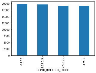
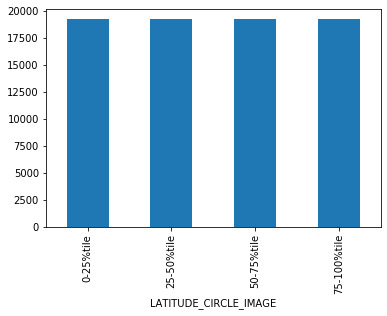
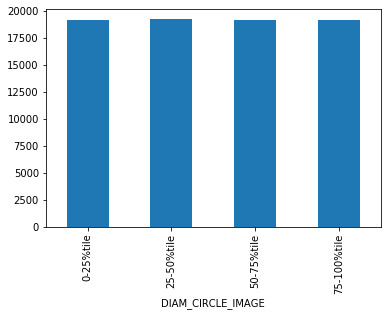
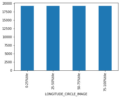
Peer-graded Assignment: Creating graphs for your data

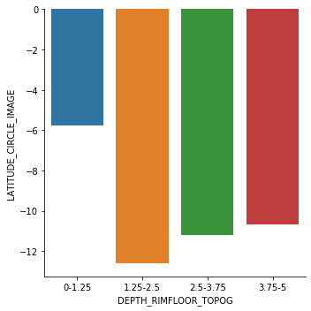
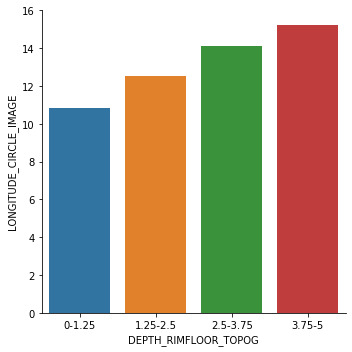
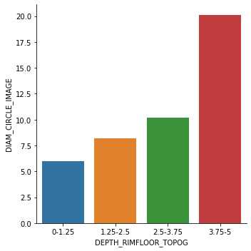
Objective of this study is to create univariate to understand counts of response variable and explanatory variables. Crater depth ('DEPTH_RIMFLOOR_TOPOG) has been chosen as response variable and “'LATITUDE_CIRCLE_IMAGE”, “LONGITUDE_CIRCLE_IMAGE” & “DIAM_CIRCLE_IMAGE”are chosen as explanatory variables. Univariate and bivariate plots are generated for relationship interpretation among variables.

Summary:

Univariate plots on explanatory variables are presented in first three Figure presented the subsequent report. Univariate plots show that all three explanatory variables are almost equally distributed among 4 quartiles. Bivariate plots are generated to understand the association between explanatory and response variables. Last three figure represent relationship of response variable with all three explanatory variables. Bivariate plot signifies variability of response among 4 quartiles.

Details of the Python script used in this study is documented towards the end of this document.

PYTHON SCRIPT

"""

# -*- coding: utf-8 -*-

"""

Spyder Editor

This is a temporary script file.

"""

import pandas as pd

import numpy as np

import seaborn as sns

import matplotlib.pyplot as plt

# load Mars crater dataset

data = pd.read_csv('marscrater_pds.csv',low_memory=False)

pd.set_option('display.float_format', lambda x:'%f'%x)

# display summary statistics about the data

print("Statistics for RIM DEPTH raw data")

print(data['DEPTH_RIMFLOOR_TOPOG'].describe())

# subset data for crater depth, negative and zero data's are ignored

data_neg = data[(data['DEPTH_RIMFLOOR_TOPOG']<0)]

data_datum = data[(data['DEPTH_RIMFLOOR_TOPOG']==0)]

data_depth = data[(data['DEPTH_RIMFLOOR_TOPOG']>0)]

print("Statistics for crater depth")

print(data_depth['DEPTH_RIMFLOOR_TOPOG'].describe())

####Univariate plot,LATITUDE_CIRCLE_IMAGE#####################

sub0 = data_depth.copy()

sub0['LATITUDE_CIRCLE_IMAGE'] = pd.qcut(sub0.LATITUDE_CIRCLE_IMAGE, 4, labels=["0-25%tile","25-50%tile","50-75%tile","75-100%tile"])

print("Counts for crater LATITUDE splitted in 4 groups: 0-25%tile, 25-50%tile, 50-75%tile, 75-100%tile")

sub0grp = sub0.groupby('LATITUDE_CIRCLE_IMAGE').size()

print(sub0grp)

sub0grp.plot.bar()

#####Univariate plot,LONGITUDE_CIRCLE_IMAGE##########################

sub1 = data_depth.copy()

sub1['LONGITUDE_CIRCLE_IMAGE'] = pd.qcut(sub1.LONGITUDE_CIRCLE_IMAGE, 4, labels=["0-25%tile","25-50%tile","50-75%tile","75-100%tile"])

print("Counts for crater LONGITUDE splitted in 4 groups: 0-25%tile, 25-50%tile, 50-75%tile, 75-100%tile")

sub1grp = sub1.groupby('LONGITUDE_CIRCLE_IMAGE').size()

print(sub1grp)

sub1grp.plot.bar()

###Univariate plot,DIAM_CIRCLE_IMAGE######################

sub3 = data_depth.copy()

sub3['DIAM_CIRCLE_IMAGE'] = pd.qcut(sub3.DIAM_CIRCLE_IMAGE, 4, labels=["0-25%tile","25-50%tile","50-75%tile","75-100%tile"])

print("Counts for crater DIAM splitted in 4 groups: 0-25%tile, 25-50%tile, 50-75%tile, 75-100%tile")

sub3grp = sub3.groupby('DIAM_CIRCLE_IMAGE').size()

print(sub3grp)

sub3grp.plot.bar()

######### Univariate plot,DEPTH_RIMFLOOR ##########

sub2 = data_depth.copy()

sub2['DEPTH_RIMFLOOR_TOPOG'] = pd.qcut(sub2.DEPTH_RIMFLOOR_TOPOG, 4, labels=["0-1.25","1.25-2.5","2.5-3.75","3.75-5"])

print("Counts for age splitted in 4 groups: 0-1.25, 1.25-2.5, 2.5-3.75, 3.75-5")

sub2grp = sub2.groupby('DEPTH_RIMFLOOR_TOPOG').size()

print(sub2grp)

sub2grp.plot.bar()

##Bivariate plot for association of crater depth with crater latitude

sns.factorplot(x='DEPTH_RIMFLOOR_TOPOG', y='LATITUDE_CIRCLE_IMAGE', data=sub2, kind="bar", ci=None)

plt.xlabel('DEPTH_RIMFLOOR_TOPOG')

plt.ylabel('LATITUDE_CIRCLE_IMAGE')

###Bivariate plot for association of crater depth with crater longitude

sns.factorplot(x='DEPTH_RIMFLOOR_TOPOG', y='LONGITUDE_CIRCLE_IMAGE', data=sub2, kind="bar", ci=None)

plt.xlabel('DEPTH_RIMFLOOR_TOPOG')

plt.ylabel('LONGITUDE_CIRCLE_IMAGE')

# #Bivariate plot for association of crater depth with crater diameter

sns.factorplot(x='DEPTH_RIMFLOOR_TOPOG', y='DIAM_CIRCLE_IMAGE', data=sub2, kind="bar", ci=None)

plt.xlabel('DEPTH_RIMFLOOR_TOPOG')

plt.ylabel('DIAM_CIRCLE_IMAGE')

0 notes

subrotonayak · 4 years

Text

Peer-graded Assignment: Making Data Management Decisions

Objective of this study is to study the decisions about identified data variables. Crater depth statistics helped to identify data abnormality and helped to clear the dataset to be used. Crater depth with negative value and zeros are not used for this study. First data are cleaned to have logical crater depth and associated variables. Variable’s identified for this study are Crater latitude circle, crater longitude circle and crater diameter.

Insights on variables

Distribution counts and frequencies of each variables are calculated to fletch insights from variables. New variables are generated from the existing variables. Details calculations are presented in subsequent document. Python script is also embedded in this content. Followings are the key insights from variables:

1. Crater latitude circle (LATITUDE_CIRCLE_IMAGE) and Crater longitude circle (LONGITUDE_CIRCLE_IMAGE) is ranged from positive value to negative value. Negative and positive signifies direction of data and hence they are considered as new variables

New variable creation from variables

As Crater latitude circle (LATITUDE_CIRCLE_IMAGE) and Crater longitude circle (LONGITUDE_CIRCLE_IMAGE) had data ranges from positive value to negative value, these two variables are segregated to generates new variables. Crater diameter (DIAM_CIRCLE_IMAGE) is range only positive value and hence no new variable is generated from this variable. Details of the findings are documented in the following content. Python script is also embedded in this content

Followings are the key finding from the distribution study:

1. Segregated positive and negative of each variable (LATITUDE_CIRCLE_IMAGE & LONGITUDE_CIRCLE_IMAGE) to create new variables.

Summary of Frequency distributions:

Frequency distribution of all three variables are calculated to understand the data patters and subsequent data segregation to create new variables. Details of the findings on frequency distributions are documented in the following content. Python script is also embedded in this content. Followings re the key finding from the distribution study:

1. Distribution of Crater latitude circle (LATITUDE_CIRCLE_IMAGE) signifies that its value can vary from -68.6 to +50.4. Data sets are segregated in 5 bins to understand distributions. Majority of the data is falling in the range -20.9 to 2.8. Details of the study presented in the subsequent content.

2. Distribution of Crater longitude circle (LONGITUDE_CIRCLE_IMAGE) signifies that its value can vary from -174.1 to 169.2. Data sets are segregated in 5 bins to understand distributions. Majority of the data is falling in the range -36.5 to 32.0. Details of the study presented in the subsequent content.

3. Distribution of Crater diameter (DIAM_CIRCLE_IMAGE) signifies that its value can vary from -34.7 to 312.4. Data sets are segregated in 5 bins to understand distributions. Majority of the data is falling in the range 34.7 to 90.4. Details of the study presented in the subsequent content.

Statistics for RIM DEPTH raw data

count 384343.000000

mean 0.075838

std 0.221518

min -0.420000

25% 0.000000

50% 0.000000

75% 0.000000

max 4.950000

Counts for deep crater Depth

counts percentages

4.750000 1 0.015385

2.720000 1 0.015385

3.030000 1 0.015385

2.940000 1 0.015385

2.560000 4 0.061538

2.590000 3 0.046154

2.870000 1 0.015385

4.010000 1 0.015385

2.620000 2 0.030769

4.720000 1 0.015385

Statistics for deep crater

count 65.000000

mean 2.913846

std 0.533141

min 2.510000

25% 2.560000

50% 2.760000

75% 2.980000

max 4.950000

Frequency for Latitude circle

Range Counts

(-68.61800000000001, -44.707] 8

(-44.707, -20.916] 13

(-20.916, 2.875] 24

(2.875, 26.666] 12

(26.666, 50.457] 8

Percentage for Latitude circle

Range Percentage

(-68.61800000000001, -44.707] 12.307692

(-44.707, -20.916] 20.000000

(-20.916, 2.875] 36.923077

(2.875, 26.666] 18.461538

(26.666, 50.457] 12.307692

Frequency for Longitude circle

Range Counts

(-68.61800000000001, -44.707] 8

(-44.707, -20.916] 13

(-20.916, 2.875] 24

(2.875, 26.666] 12

(26.666, 50.457] 8

Percentage for Longitude circle

Range Percentage

(-174.18, -105.217] 6.153846

(-105.217, -36.598] 26.153846

(-36.598, 32.02] 38.461538

(32.02, 100.639] 20.000000

(100.639, 169.258] 9.230769

Frequency for Crater Diameter

Range Counts

(34.732, 90.496] 45

(90.496, 145.982] 14

(145.982, 201.468] 3

(201.468, 256.954] 2

(256.954, 312.44] 1

Percentage for Crater Diameter

Range Percentage

(34.732, 90.496] 69.230769

(90.496, 145.982] 21.538462

(145.982, 201.468] 4.615385

(201.468, 256.954] 3.076923

(256.954, 312.44] 1.538462

PYTHON SCRIPT

"""

Spyder Editor

This is a temporary script file.

"""

import pandas as pd

import numpy as np

import seaborn as sns

import matplotlib.pyplot as plt

# load Mars crater dataset

data = pd.read_csv('marscrater_pds.csv',low_memory=False)

pd.set_option('display.float_format', lambda x:'%f'%x)

# display summary statistics about the data

print("Statistics for RIM DEPTH raw data")

print(data['DEPTH_RIMFLOOR_TOPOG'].describe())

# subset data for crater depth, negative and zero data's are ignored

data_neg = data[(data['DEPTH_RIMFLOOR_TOPOG']<0)]

data_datum = data[(data['DEPTH_RIMFLOOR_TOPOG']==0)]

data_depth = data[(data['DEPTH_RIMFLOOR_TOPOG']>0)]

# subset data for deep crater

deep_crater = data[(data['DEPTH_RIMFLOOR_TOPOG']>2.5)]

# identifying counts of deep crater depth

print("Counts for deep crater Depth")

crater_depth_freq = pd.concat(dict(counts = deep_crater["DEPTH_RIMFLOOR_TOPOG"].value_counts(sort=False, dropna=False), percentages = deep_crater["DEPTH_RIMFLOOR_TOPOG"].value_counts(sort=False, dropna=False, normalize=True)), axis=1)

print(crater_depth_freq.head(10))

# Rimfloor depth statistics

print("Statistics for deep crater")

print(deep_crater['DEPTH_RIMFLOOR_TOPOG'].describe())

#################################################################################

# LATITUDE_CIRCLE_IMAGE

#################################################################################

# frequency and percentage distritions for crater LATITUDE_CIRCLE_IMAGE (laci)

print('Frequency for Latitude circle')

print('Range Counts')

laci = deep_crater['LATITUDE_CIRCLE_IMAGE'].value_counts(sort=False,bins=5)

print(laci)

print('Percentage for Latitude circle')

print('Range Percentage')

placi = deep_crater['LATITUDE_CIRCLE_IMAGE'].value_counts(sort=False,bins=5,normalize=True)*100

print(placi)

#Creating new variables

lci_positive = deep_crater[(deep_crater['LATITUDE_CIRCLE_IMAGE'] > 0)]

lci_negative = deep_crater[(deep_crater['LATITUDE_CIRCLE_IMAGE'] < 0)]

#################################################################################

# LONGITUDE_CIRCLE_IMAGE

#################################################################################

# frequency and percentage distritions for crater LONGITUDE_CIRCLE_IMAGE (loci)

print('Frequency for Longitude circle')

print('Range Counts')

loci = deep_crater['LONGITUDE_CIRCLE_IMAGE'].value_counts(sort=False,bins=5)

print(laci)

print('Percentage for Longitude circle')

print('Range Percentage')

ploci = deep_crater['LONGITUDE_CIRCLE_IMAGE'].value_counts(sort=False,bins=5,normalize=True)*100

print(ploci)

#Creating new variables

loci_positive = deep_crater[(deep_crater['LONGITUDE_CIRCLE_IMAGE'] > 0)]

loci_negative = deep_crater[(deep_crater['LONGITUDE_CIRCLE_IMAGE'] < 0)]

############################################################################

# DIAM_CIRCLE_IMAGE

###########################################################################

# frequency and percentage distritions for Crater Diameter (dci)

print('Frequency for Crater Diameter')

print('Range Counts')

dci = deep_crater['DIAM_CIRCLE_IMAGE'].value_counts(sort=False,bins=5)

print(dci)

print('Percentage for Crater Diameter')

print('Range Percentage')

pdci = deep_crater['DIAM_CIRCLE_IMAGE'].value_counts(sort=False,bins=5,normalize=True)*100

print(pdci)

0 notes

subrotonayak · 5 years

Text

Peer-graded Assignment: Running Your First Program

Output with Frequency Tables at Crater depth for Crater latitude circle, crater longitude circle and crater diameter

Summary of Frequency Distributions

Crater depth statistics helped to identify data abnormality and helped to clear the dataset for frequency distribution. Statistics of crater depth helped to identify unrealistic crater depth and python scrip is used to remove those unrealistic data and clear the dataset. Variables identified for this study are “LATITUDE_CIRCLE_IMAGE”, “LONGITUDE_CIRCLE_IMAGE” and “DIAM_CIRCLE_IMAGE”. Frequency distributions are studied for each variable separately. Details of the findings are documented in the following content. Python script is also embedded in this content. Followings re the key finding from the distribution study:

1. Distribution of Crater latitude circle (LATITUDE_CIRCLE_IMAGE) is primarily dominated by data ranges -34.979 and -17.739 and maximum crater latitude circle found to be 86.7. Details of the study presented in the subsequent content.

2. Crater longitude circle (LONGITUDE_CIRCLE_IMAGE) is primarily dominated by data ranges -0.0 and 35.999 with count of 51633. Details of the study presented in the subsequent content.

3. Main distribution of Crater circle diameter (DIAM_CIRCLE_IMAGE) is in the range of -0.164 and 117.322. Details of the study presented in the subsequent content.

Statistics for RIM DEPTH raw data

count 384343.000000

mean 0.075838

std 0.221518

min -0.420000

25% 0.000000

50% 0.000000

75% 0.000000

max 4.950000

Counts for Rimfloor Depth

counts percentages

0.00 307529 0.800163

2.00 14 0.000036

0.22 1189 0.003094

0.19 1363 0.003546

0.43 684 0.001780

0.13 1763 0.004587

0.09 2008 0.005225

1.43 38 0.000099

0.27 1004 0.002612

0.44 698 0.001816

Statistics for RIM DEPTH with clear data

count 384333.000000

mean 0.075841

std 0.221518

min 0.000000

25% 0.000000

50% 0.000000

75% 0.000000

max 4.950000

Statistics for variable latitude circle

count 384333.000000

mean -7.199614

std 33.608671

min -86.700000

25% -30.935000

50% -10.079000

75% 17.222000

max 85.702000

Counts for Latitude circle

counts percentages

32.000 2 0.000005

2.000 1 0.000003

0.000 7 0.000018

-2.000 4 0.000010

-32.000 4 0.000010

-28.335 3 0.000008

-24.670 3 0.000008

-0.217 1 0.000003

-69.018 1 0.000003

-72.738 1 0.000003

Frequency for Latitude circle

(-86.873, -69.46] 8234

(-69.46, -52.22] 27317

(-52.22, -34.979] 45391

(-34.979, -17.739] 76206

(-17.739, -0.499] 74363

(-0.499, 16.741] 55366

(16.741, 33.981] 48216

(33.981, 51.222] 28934

(51.222, 68.462] 16474

(68.462, 85.702] 3832

Percentage for Latitude circle

(-86.873, -69.46] 2.142413

(-69.46, -52.22] 7.107638

(-52.22, -34.979] 11.810331

(-34.979, -17.739] 19.828118

(-17.739, -0.499] 19.348586

(-0.499, 16.741] 14.405737

(16.741, 33.981] 12.545371

(33.981, 51.222] 7.528367

(51.222, 68.462] 4.286387

(68.462, 85.702] 0.997052

Cumulative frequency of Latitude circle

[8234, 35551, 80942, 157148, 231511, 286877, 335093, 364027, 380501, 384333]

Cumulative percentage for Latitude circle

[2.1424129595949344, 9.25005138772887, 21.060382532855623, 40.88850033694739, 60.23708606859156, 74.64282276047074, 87.18819357172036, 94.71656089901205, 99.00294796439546, 100.0]

Statistics for variable longitude circle

count 384333.000000

mean 10.128091

std 96.642183

min -179.997000

25% -58.830000

50% 12.739000

75% 89.277000

max 179.997000

Counts for Longitude circle

counts percentages

64.000 2 0.000005

2.000 5 0.000013

-0.125 1 0.000003

0.000 3 0.000008

102.076 3 0.000008

102.424 2 0.000005

73.262 2 0.000005

47.992 2 0.000005

123.252 1 0.000003

-73.912 3 0.000008

Frequency for Longitude circle

(-180.358, -143.998] 33164

(-143.998, -107.998] 21211

(-107.998, -71.999] 27960

(-71.999, -35.999] 43170

(-35.999, 0.0] 48433

(0.0, 35.999] 51633

(35.999, 71.999] 42175

(71.999, 107.998] 42282

(107.998, 143.998] 39432

(143.998, 179.997] 34873

Percentage for Longitude circle

(-180.358, -143.998] 8.628975

(-143.998, -107.998] 5.518912

(-107.998, -71.999] 7.274941

(-71.999, -35.999] 11.232447

(-35.999, 0.0] 12.601832

(0.0, 35.999] 13.434444

(35.999, 71.999] 10.973557

(71.999, 107.998] 11.001397

(107.998, 143.998] 10.259853

(143.998, 179.997] 9.073642

Cumulative frequency of Longitude circle

[8234, 35551, 80942, 157148, 231511, 286877, 335093, 364027, 380501, 384333]

Cumulative percentage for Longitude circle

[2.1424129595949344, 9.25005138772887, 21.060382532855623, 40.88850033694739, 60.23708606859156, 74.64282276047074, 87.18819357172036, 94.71656089901205, 99.00294796439546, 100.0]

Statistics for Crater Diameter

count 384333.000000

mean 3.556186

std 8.591304

min 1.000000

25% 1.180000

50% 1.530000

75% 2.550000

max 1164.220000

Counts for Crater Diameter

counts percentages

64.000 2 0.000005

2.000 5 0.000013

-0.125 1 0.000003

0.000 3 0.000008

102.076 3 0.000008

102.424 2 0.000005

73.262 2 0.000005

47.992 2 0.000005

123.252 1 0.000003

-73.912 3 0.000008

Frequency for Crater Diameter

(-0.164, 117.322] 384150

(117.322, 233.644] 148

(233.644, 349.966] 24

(349.966, 466.288] 6

(466.288, 582.61] 2

(582.61, 698.932] 1

(698.932, 815.254] 0

(815.254, 931.576] 0

(931.576, 1047.898] 0

(1047.898, 1164.22] 2

Percentage for Crater Diameter

(-0.164, 117.322] 99.952385

(117.322, 233.644] 0.038508

(233.644, 349.966] 0.006245

(349.966, 466.288] 0.001561

(466.288, 582.61] 0.000520

(582.61, 698.932] 0.000260

(698.932, 815.254] 0.000000

(815.254, 931.576] 0.000000

(931.576, 1047.898] 0.000000

(1047.898, 1164.22] 0.000520

Cumulative frequency of Crater Diameter

[8234, 35551, 80942, 157148, 231511, 286877, 335093, 364027, 380501, 384333]

Cumulative percentage for Crater Diameter

[2.1424129595949344, 9.25005138772887, 21.060382532855623, 40.88850033694739, 60.23708606859156, 74.64282276047074, 87.18819357172036, 94.71656089901205, 99.00294796439546, 100.0]

Python Script:

Spyder Editor

This is a temporary script file.

"""

import pandas as pd

import numpy as np

import seaborn as sns

import matplotlib.pyplot as plt

# load Mars crater dataset

data = pd.read_csv('marscrater_pds.csv',low_memory=False)

#setting variables you will be working with to numeric

#data['CRATER_ID'] = data['CRATER_ID'].convert_objects(convert_numeric=True)

#data['LATITUDE_CIRCLE_IMAGE'] = data['LATITUDE_CIRCLE_IMAGE'].convert_objects(convert_numeric=True)

#data['LONGITUDE_CIRCLE_IMAGE'] = data['LONGITUDE_CIRCLE_IMAGE'].convert_objects(convert_numeric=True)

#data['DIAM_CIRCLE_IMAGE'] = data['DIAM_CIRCLE_IMAGE'].convert_objects(convert_numeric=True)

#data['DEPTH_RIMFLOOR_TOPOG'] = data['DEPTH_RIMFLOOR_TOPOG'].convert_objects(convert_numeric=True)

# display summary statistics about the data

print("Statistics for RIM DEPTH raw data")

print(data['DEPTH_RIMFLOOR_TOPOG'].describe())

# subset data for deep crater based on summary statistics

sub = data[(data['DEPTH_RIMFLOOR_TOPOG']>=0)]

#make a copy of my new subsetted data

data_shorted = sub.copy()

# identifying counts of top Rimfloor depth

print("Counts for Rimfloor Depth")

DEPTH_RIMFLOOR_TOPOG_freq = pd.concat(dict(counts = data_shorted["DEPTH_RIMFLOOR_TOPOG"].value_counts(sort=False, dropna=False), percentages = data_shorted["DEPTH_RIMFLOOR_TOPOG"].value_counts(sort=False, dropna=False, normalize=True)), axis=1)

print(DEPTH_RIMFLOOR_TOPOG_freq.head(10))

# Rimfloor depth statistics

print("Statistics for RIM DEPTH with clear data")

print(data_shorted['DEPTH_RIMFLOOR_TOPOG'].describe())

#################################################################################

# LATITUDE_CIRCLE_IMAGE

#################################################################################

# Analysis variable latitude circle

print("Statistics for variable latitude circle")

print(data_shorted['LATITUDE_CIRCLE_IMAGE'].describe())

# identifying counts of top 10 latitude circle

print("Counts for Latitude circle")

LATITUDE_CIRCLE_IMAGE_freq = pd.concat(dict(counts = data_shorted["LATITUDE_CIRCLE_IMAGE"].value_counts(sort=False, dropna=False), percentages = data_shorted["LATITUDE_CIRCLE_IMAGE"].value_counts(sort=False, dropna=False, normalize=True)), axis=1)

print(LATITUDE_CIRCLE_IMAGE_freq.head(10))

# frequency and percentage distritions for crater LATITUDE_CIRCLE_IMAGE (laci)

print('Frequency for Latitude circle')

laci = data_shorted['LATITUDE_CIRCLE_IMAGE'].value_counts(sort=False,bins=10)

print(laci)

print('Percentage for Latitude circle')

placi = data_shorted['LATITUDE_CIRCLE_IMAGE'].value_counts(sort=False,bins=10,normalize=True)*100

print(placi)

# cumulative frequency and cumulative percentage for LATITUDE_CIRCLE_IMAGE

cfplaci=[] # Cumulative Frequency

cpplaci=[] # Cumulative Percentage

cf=0

cp=0

for freq in laci:

cf=cf+freq

cfplaci.append(cf)

pf=cf*100/len(data_shorted)

cpplaci.append(pf)

print('Cumulative frequency of Latitude circle')

print(cfplaci)

print('Cumulative percentage for Latitude circle')

print(cpplaci)

#################################################################################

# LONGITUDE_CIRCLE_IMAGE

#################################################################################

# Analysis variable longitude circle

print("Statistics for variable longitude circle")

print(data_shorted['LONGITUDE_CIRCLE_IMAGE'].describe())

# identifying counts of top 10 Longitude circle

print("Counts for Longitude circle")

LONGITUDE_CIRCLE_IMAGE_freq = pd.concat(dict(counts = data_shorted["LONGITUDE_CIRCLE_IMAGE"].value_counts(sort=False, dropna=False), percentages = data_shorted["LONGITUDE_CIRCLE_IMAGE"].value_counts(sort=False, dropna=False, normalize=True)), axis=1)

print(LONGITUDE_CIRCLE_IMAGE_freq.head(10))

# frequency and percentage distritions for crater Longitude circle (loci)

print('Frequency for Longitude circle')

loci = data_shorted['LONGITUDE_CIRCLE_IMAGE'].value_counts(sort=False,bins=10)

print(loci)

print('Percentage for Longitude circle')

ploci = data_shorted['LONGITUDE_CIRCLE_IMAGE'].value_counts(sort=False,bins=10,normalize=True)*100

print(ploci)

# cumulative frequency and cumulative percentage for LONGITUDE_CIRCLE_IMAGE

cfploci=[] # Cumulative Frequency

cpploci=[] # Cumulative Percentage

cf=0

cp=0

for freq in laci:

cf=cf+freq

cfploci.append(cf)

pf=cf*100/len(data_shorted)

cpploci.append(pf)

print('Cumulative frequency of Longitude circle')

print(cfploci)

print('Cumulative percentage for Longitude circle')

print(cpploci)

# DIAM_CIRCLE_IMAGE

# Analysis variable longitude circle

print("Statistics for Crater Diameter")

print(data_shorted['DIAM_CIRCLE_IMAGE'].describe())

# identifying counts of top 10 Crater Diameter

print("Counts for Crater Diameter")

DIAM_CIRCLE_IMAGE_freq = pd.concat(dict(counts = data_shorted["DIAM_CIRCLE_IMAGE"].value_counts(sort=False, dropna=False), percentages = data_shorted["DIAM_CIRCLE_IMAGE"].value_counts(sort=False, dropna=False, normalize=True)), axis=1)

print(LONGITUDE_CIRCLE_IMAGE_freq.head(10))

# frequency and percentage distritions for Crater Diameter (dci)

print('Frequency for Crater Diameter')

dci = data_shorted['DIAM_CIRCLE_IMAGE'].value_counts(sort=False,bins=10)

print(dci)

print('Percentage for Crater Diameter')

pdci = data_shorted['DIAM_CIRCLE_IMAGE'].value_counts(sort=False,bins=10,normalize=True)*100

print(pdci)

# cumulative frequency and cumulative percentage for Crater Diameter

cfpdci=[] # Cumulative Frequency

cppdci=[] # Cumulative Percentage

cf=0

cp=0

for freq in laci:

cf=cf+freq

cfpdci.append(cf)

pf=cf*100/len(data_shorted)

cppdci.append(pf)

print('Cumulative frequency of Crater Diameter')

print(cfpdci)

print('Cumulative percentage for Crater Diameter')

print(cppdci)

0 notes