ryogrid - Tumblr blog

ryogrid · 2 years ago

Text

Hentai Diffusionでエッチな画像を綺麗に生成するノウハウを見つけたので共有する（生成画像には制約あり）

世のスケベの皆さんこんばんわ。

Windows 10 Homeのマシンで簡単に環境構築出来て、生成できたものも想像以上にクオリティの高いものだったので情報共有します。

注意点（１）

本記事の内容を閲覧したものの行動により生じた損害等について筆者は一切の責任を負いかねますので、ご了承ください

本記事が提供する情報を利用する場合は、自己責任で行う必要があります

注意点（２）

NVIDIA製のグラフィックボードを搭載しているマシンでないと、おそらく厳しい戦いになると思います

AMDのRADEONを使う方法や、CPUで頑張る方法もあるようですがこの記事ではそのあたりのやり方には触れません

また、性能があまりにも低いと動かないか、画像生成にものすごく時間がかかったりするかもしれませんが、その点はご承知下さい

筆者はNVIDIA GeForce GTX 1660 Super というグラボを搭載したマシンで動かしていて、Sampling Stepsが120、画像サイズ512x512pxで一枚生成するのに一分半ほどかかっています

生成時間は（主に）Sampling

Stepsというパラメータの大きさや画像サイズによるので、そこらへんをよしなに下げれば筆者が利用しているグラボよりスペックの低いボードでもなんとかなる場合も多いと思います

注意点（３）

後述しますが、特定の容姿の人物に関しては綺麗に生成ができまして、そこのところがこの記事のキモでもあるのですが、任意のキャラや好きな容姿の女性・男性について綺麗に生成できるかは分からない、というか、多分この記事の手順だけでは無理だと思います

ただ、筆者はあまり試していませんが、scriptの内容である程度は容姿を変えられるのではないかと思うので、頑張りたい方は頑張ってみて下さい

注意点（4）

筆者筆者はディープラーニングと呼ばれる手法はある程度知っていますし、同手法を用いたプログラ��プログラムをいくらか書いてみたりした経験はありますが、画像生成系などはGANってどんなもの？とか前に技術記事を読んだくらいで、正直Stable Diffusionが中で何やっているのか、などよくは知りません

単に使うだけの話でも情報収集はさほどしていません

要は、雰囲気でStable Diffusionしている程度の人なので、細かいツッコミなどはご勘弁いただければありがたく〇刀乙

Stable Diffusion web UI(AUTOMATIC1111版)のセットアップ

まず、下の記事からリンクなど辿って、"Stable Diffusion web UI(AUTOMATIC1111版)"というやつをセットアップしましょう

"画像生成AI「Stable Diffusion」でいろいろ特化した使えるモデルデータいろいろまとめ - GIGAZINE"

これから導入するのであれば、当面は細かいバージョンは気にしなくて良いと思われますが、一応私が利用している利用しているものはv1.3.8のようです

グラボの搭載VRAM量に合わせて少しファイルを書き換えたりなんだり

下のページなどを参照のこと

"VRAM 4GBでStable Diffusion(Automatic1111)を動かす - note"

グラボが半精度浮動小数点演算をサポートしていない場合

そのままだとうまく動きません・・・

は？半精度うんたら？？？という感じかもしれませんが、まあ、とにかくGTX 16XXシリーズはこの問題をピンポイントで踏んでいて、下のオプションを上のページで解説しているのと同様のところに追加する必要がありました

"--precision full --no-half"

Stable Diffusionの利用をさしてリテラシがなくとも、時間かけずともできるようweb-uiなどのもろもろを有志の方々が整備してくれているわけですが、最終的に内部で行われている処理はまあ言うて難しいことなので、仕方がないですね

いろいろ整備してくれている皆さんへの感謝の気持ちを忘れないようにしつつスケベの道を進んでいきましょう

Stable Diffusionの派生モデルであるHentai Diffusionを利用するよう設定する

ここまでやればStable Diffusionでの画像生成はできるようになっているのではないかと思いますが、この記事のゴールはそこではありません

上に貼ったGIGAZINEさんの記事でも紹介されているHentai Diffusionというやつで画像生成をするようにします

ただ、元々ホストしていたところからは入手できなくなっているようなので、インターネッツの世界を放浪して見つけましょう

RD1212.ckpt というファイルだけあれば良いです

入手したらStable Diffusion web UIのmodelsディレクトリに配置します

続いて、Web UI上のSettingsのタブで開いた画面の中に"Stable Diffusion checkpoint" というやつがあるので、そこのドロップダウンで RD1212.ckpt を選択

"Allowed categories for random artists selection when using the Roll button" とか書いてあるところがあるので、"anime"を選択しておきます

画面上方のApply settingsというやつを押して設定を保存します

"Shishiro Botan" さんについて作成されたembeddingのデータを導入する

下のサイトから "Shishiro Botan" さんについてembedding?ファインチューニング？などと呼ばれる追加学習的なことをして作られたモデルデータ（の一部に相当？する）ptファイルをダウンロードします

"viper1 / stable-diffusion-embeddings・GitLab"

ダウンロードしたファイルはckptファイルを配置した際と同様にembeddingsディレクトリの中に配置して下さい

ptファイルについては特に設定せずとも勝手にロードされるようです

この"Shishiro Botan"さんについて学習したembeddingのデータが大変良くできており"Shishiro Botan"さん風の画像を生成するに限っては、想定していた以上に綺麗な画像が生成できている、と少なくとも筆者は認識しています

画像を生成する

あとはお好きにどうぞ

参考までに以下のpromptを入れておくと良さげっぽいので書いておきます

普通のところ

((nsfw)),detailed blushing [anime girl:botan-50000:.05] in (服装とかについて適宜書いておく),(pixiv),(((sex))),(solo),(a perfect face),(intense shadows), ((sharp focus)), ((hentai)),masterpiece

Negative Prompt（と呼ぶのであってた・・・はず）

((poorly drawn face)), ((poorly drawn hands)), ((poorly drawn feet)), (disfigured), ((out of frame)), (((long neck))), (big ears), ((((tiling)))), ((bad hands)), (bad art)

Stable Diffusionを利用するにあたって参考になったサイト

"Waifu Diffusion で効率的に画像を生成する"

生成した画像参考

あまりにアレな画像をアレするのはアレかと思ったので、ほどほどのスケベに抑えていますが、クオリティのほどは伝わるのではないかと思います

image1

image2

画像ファイルへの直リ��はお行儀が悪いですが、・・・すみません・・・

#stable diffusion #hentai diffusion

0 notes

ryogrid · 4 years ago

Text

Test of reblog

Python Implementation of FX System Trading Agent with Deep Reinforcement Learning (DQN)

Hi, I’m ryo_grid a.k.a. Ryo Kanbayashi.

I implemented a trading agent (with decent performance) with deep reinforcement learning (DQN) to simulate automated forex trading (FX) as an practice for learning how to apply deep reinforcement learning to time series data.

This work have done with time of 20% rule system at my place of work partially: Ory Laboratory inc .

In this article, I introduce details about my implementation and some ideas about deep reinforcement learned trade agent. My implementation is wrote with Python and uses Keras (TensorFlow) for implementing deep learning based model.

Implementation

Papers referenced (hereinafter called to “the paper”)

“Deep Reinforcement Learning for Trading”, Zihao Zhang & Stefan Zohren & Stephen Roberts, 2019 . papers 1911.10107, arXiv.org.

State

Current price (Close)

Past returns

The difference between the price at time t and the price at time t, which corresponds to the episode

The method proposed in the paper is not intended for FX only. So, as an example, if we consider the case of stocks, I thought that we can interpret the price change as a return

4 features. 1 year, 1 month, 2 months, 3 months

These are normalized by the square root of the number of days in the period and the exponentially wighted moving starndard deviation (EMSD) in the last 60 days

(In my implementation, I replaced one day to a half-day, so a number used on calculation is double the number of days)

About EMSD in Wikipedia

For more information, please see the paper and my implementation

Moving Average Convergence Divergence (MACD)

It seems to mean the same thing as what is commonly known, but the method of calculation seems to be different, so please refer to the formula in the paper and my implementation

Relative Strength Index (RSI)

It looks past 30 days

Later features are added by me (I replaced LSTM layers which handle multiple time series data to Dense layers. So, I added several technical indicators as summary data for historical price transition)

Change ratio in price between a price of t and price of t-1

Several Technical Indicators

Moving Avarage (MA)

MA Deviation Rate

First line value of the Bollinger Bands

Seconde line value of the Bollinger Band

Percentage Price Oscilator (PPO)

Chande Momentum Oscillator (CMO)

volatility

Exponentially wighted moving starndard deviation (EMSD) in the last 60 days

Same as the value used in calculating the feature “Past returns”, and same as the value used in calculating the reward

Action

Sell, Do nothing, Buy

Actions are replesented as Sell = -1, Do nothing = 0, Buy = 1

Environment buys and sells corresponding to the selected action, puts the value shown above corresponding to the action into the reward formula, and returns the value to agent

Do nothing: do nothing

Buy: close a short position and open a long position If having a long position. If not, do nothing

Sell: close a short position and open the short position If having a short position. If not, do nothing

　　　The formula for calculating reward

Reward

Calculating formula

Calculating fomula is one shown above

Each constant and variable

A{t}: the value corresponding to the action selected at time t. The value is: Sell = -1, Do nothing = 0, Buy = 1. When it used in the calculation, t indicates the time of the current episode. The formula for reward uses the actions selected at t-1 episode and t-2 episode. But A{t} which is selected at current episode is not used

μ: in the case of FX, it is equivalent to the number of currencies to be purchased. The paper says the was set to 1

σ{t}: volatility at time t. See the paper and serious implementation for the calculation

σ{tgt}: I honestly don’t understand much about this. The value must be a certain percentage of the value of return for a particular period of time (not constant value) accordint to refereed papers from the paper. But performance was bad when the definition is used. So I checked the range of values that σ{t} and I fixed it to 5.0

p{t}: price at time t without considering the spread

r{t}: p{t} - p{t-1}

bp: the percentage of transaction fees, which in the case of FX is payed as spread. In the my implementation, if there was a spread of 0.003 Yen per Dollar when 1doller = 100Yen, the valuation loss is assumed to be 0.0015 Yen for one way. So I fixed bp to 0.0015

Interpretation of the reward formula in broad terms

The basic idea is to learn appropriate actions corresponding to input features from the results of transactions in the training data (I recognize that this is essentially the same as forex prediction, etc.)

However, instead of simply using trading results as a reward, the risk of holding a position represented with the recent volatility is considered and the reward is scaled with the risk value (in the paper, this may be a method that is applied to portfolio management, etc.)

In calculating the reward at a episode in time t, informatoin of A{t} selected in time t is not used. It seems strange. However certain percentage of the rewards in next episode is added (sometimes positive, sometimes negative) due to Q-learning update equation. And reward of next episode in time t+1 is mainly determined from result of a transaction corresponding to A{t}. So there is no problem.

Interpretation of specific expressions

Fomula in box brackets corresponds to the change in holding status of a long or short position for one currency bought and sold one episode ago (even if there is no change in the position). And μ corresponds to the number of currencies bought and sold

The first item in the box brackets evaluates the action one episode earlier A{t-1}. A{t-1} varies in {-1, 0, 1} and r{t} is the difference between the price at the time of the previous episode and the price at the current time. Therefore, the item takes a positive value if the price has gone up and a negative value if the price has gone down. Therefore A{t-1} * r{t} becomes positive value if you buy and the price goes up, and if you sell and the price goes down. It is a negative value if the trade was reversed one. In short, it represents whether the trade was correct or not. If the action was donot, A{t-1} values 0 and the value of the first item becomes 0

σ{tgt} / σ{t-1} is a coefficient for scaling the above value with volatility at t-1. In situations of low volatility, value will be higher and in high volatility, value will be lower. This causes agents to behave in such a way that it avoids trading in situations of high market volatility. It seems to me that the fractions with volatility appeared in the second item is works as same as one of first item.

On the second item, -bp * p{t-1} represents the one-way transaction cost per a currency and absolute value part represents wheter the transaction costs ware incurred in te previous episode. Therefore, multiplying them together gives the transaction cost per currency incurred in the previous episode

For the part of the second item that gives absolute value, without cossidering the scaling by volatility part, if the actions at time t-1 and t-2 were a “Sell” and “Buy” (“Buy” and “Sell”), the value is 2. The value = 2 means twice of one-way transaction costs were paid for closing a position and opening a position. “Do nothing” and “Sell” or “Buy” (even if the order is reversed) will result in a value of 1 and it means one-way cost was paied. However, in this case, there must be a case where the agent just kept the position and no cost should be incurred I think. But a one-way transaction cost was incurred on the fomula anyway. In the case of “Do nothing” and “Do nothing”, the value is 0 and no transaction cost is incurred

Differences between my implementetion and the method proposed by the paper (some of which may be my misread)

σ{tgt} for reward scaling

If I’m understanding it right (I’m not sure…), the paper seems to have a value that changes from episode to episode (not a fixed value). But when I implemented it, the performance was reducedsignificantly. So I’m using a fixed value

In calculation the standard deviation for MACD, the period of time is set to six months instead of one year

The paper seems to use volatilities calculated over the differences in price changes (the difference between sccessive two prices) as volatility. But my implementation uses vollatilities calculated over the prices direectly

I also tried to implement using volatilities calculated over the differences in price changese, but it only reduced performance, so my implementation is not using it

All replays of a iteration are done at last of the iteration (fit method of TF is called once only per iteration)

Learning period and test period

My implementation uses 13 years of data from mid-2003 to mid-2016, whereas the paper uses 15 years of data from 2005 to 2019

The paper evaluates the study period as 5 years

I’m guessing that they had it as a study/test at 5 years/5 years, and when looking at performance in the next 5 years, they moved the study period forward 5 years and re-modeled it again

Half-day, not one-day

To increase trading opportunities and the number of trade

The reason for increasing the number of trades is we think it reduces the luck factor

Batch Normalization is included (the paper doesn’t mention whether any layers are added other than the layers described)

No replaying across iterations

In my implementation, “memory” is cleared at start of each iteration and replays are random replay. Therefore the only records of the episodes used are those of the same iteration without duplication

In the paper, it is stated that the size of the memory is 5000 and replay is performed every 1000 episodes. So it seems that the contents of the memory are maintained across iterations and the replay is performed using the contents (it is not clear how the data of the episodes are selected for the replay)

The input features are normalized by scikit-learn’s StandardScaler to all of them

In the paper, it is stated that only the value of the prices are normalized

In addition, because the features of the test data must be normalized in the evaluation with test data, a instance of StandardScaler is maintained that are fitted when normalizing the features of the training data and it is used to normalize the features of the test data as well

The paper refers to the volume of transactions as a fixed number of currencies. But my implementation dynamically changes number of currencies according to amount of money agent has

In the paper, it is stated that fomula for calculation of reward value should be changed when using not fixed number of currency on each transaction to achieve compounding effect. But the formula is not changed on my implementation

Procedure for creating a model for an operational scenario

How to decide which model to use

Look at the results of backtests run periodically during learning to find just the right number of iterations before overlearning occurs

If the trade performance is stable for about a year on backtesting. Except for there is significant market trande change, it is likely that the performance will be similar. If clearly market movements and price ranges are different from the training period and the period of the test data, there is no choice but to shut down the operation

If stable result is found, you do early stopping so that you can get the model at the point. Please note that in the current implementation, the total number of iterations is used as a parameter of the gleedy method. Therefore, you can’t end execution early by reducing it. Therefore, for terminating execution, inserting code for it is necessary

If stable result does’t show up, you can change the learning period (longer or shorter)

If you want to extend the learning period, you need to increase the number of NN units and if you want to shorten it, you need to reduce it, which was found experimentally

NN’s expressive power varies with the number of units, so if it is too few, they cannot acquire even common rules in training and test data (before over-fitting begins) due to lack of representation maybe. If it is too many, early over-fitting occurs due to excessive expressive power maybe

As the performance tends to deteriorate when there is a gap between the training period and the test period, beginning of training data is moved forwards to shorten the period, and to lengthen the period, the beginning of the training period is moved backwards (if there is extra data) or the beginning of the test period is moved into the future (if you can accept to shorten the test period)

Agent trade performance simulation (USDJPY, EURJPY, GBPJPY)

Exclude about first one year for feature generation of later period and the subsequent six years (excluding non-tradeable weekends, etc) were used as training data. And remaining period (excluding non-tradeable weekends, etc) were used as test data

Since the evaluation backtest only outputs a log of option close, results graph below also shows the number of close transaction on the horizontal axis and the axis does not strictly correspond to the backtest period (periods when no closes occurred do not appear in the graph). But it almost corresponds because close operations are distributed evenly over the all period at the results below

Execution Environment

Windows 10 Home 64bit

Python 3.7.2

pip 20.0.2

pip module

tensorflow 2.1.0

scikit-learn 0.22.1

scipy 1.4.2

numpy 1.18.1

TA-Lib 0.4.17

(Though machine used for execution had GeForce GTX 1660 Super, I have disabled it at program start-up because using GPU makes learnig speed slow on the NN network scale of this model which is relatively small and I heard that fixing the seed will not be reproducible when GPU is used)

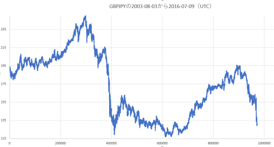
Exchange rate trends for each dataset (price of Close on dataset)

In my implementation, the price of the long position is based on p{t} + 0.0015 yen. The price of the short position is based on p{t} - 0.0015 yen. When closing, the price is the reverse of both. Taxation on trading profit is not considered.

USDJPY (2003-05-04_2016-07-09)

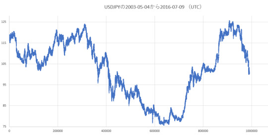
EURJPY (2003-08-03_2016-07-09)

GBPJPY (2003-08-03_2016-07-09)

Hyperparameters

Learning rate: 0.0001

Mini-batch size: 64

Traing data size: Approx. 3024 rates (half-day, approximately 6 years, not including non-tradeable days)

Number of positions (chunks of currency) that can be held: 1

NN structure: main layers are 80 units of Dense and 40 units of Dense

Dueling network is also implemented

NN structure

Backtesting results with test data for each currency pair

Backtesting is started with an initial asset of 1 million yen

The duration of the training data is about 6 years (excluding about first year of data sets).

Data of excluded first year and a little over a year is used to generate features of training period

The length of the testing period varies slightly from one another, but all of them are the last five years and a little ovaer a year (the period is continuous with the one of training data)

The following is just a case of early termination with a good number of iterations that have performed well. There are also a lot of results that are not good at all when training code progress is smaller and larger number of iterations than one of results below.

USDJPY

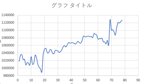
Trands when 120 iterations trained model is used

EURJPY

Trands when 50 iterations trained model is used

GBPJPY

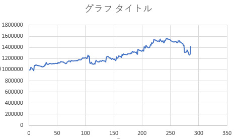
Trands when 50 iterations trained model is used

Source Code

Repository (branch): github

Source File: agent, environment

This is the code used to evaluate the dataset in USDJPY. If you want to load a file of another currency pair, you can use the codes which are commented out on environmnt’s data loading part

Trying to execute my code

If you are on Windows, you can run it as follows (standard output and error output are redirected to hoge.txt)

pip install -r requirements.py

pip install TA_Lib-0.4.17-cp37-cp37m-win_amd64.whl (required only on Windows)

python thesis_based_dqn_trade_agent.py train > hoge.txt 2>&1

My code evaluates the model every 10 iterations by backtesting at train data and test data. The bactest results are output to auto_backtest_log_{start date}.csv (log of position close only). Firstlly backtest in the period of training data runs, then backtest in the test period runs subsequently. So please use the start date and time to determine which result is you want to see

In the result csv…

Second column value is number of episode which position close occurs at (0 origin)

Ninth column value is the amount of money the agent has after closing a position

Please refer to the code to see what the other column values represent :)

A side note

Reason why LSTM is not used

It was not possible to generalize when using LSTM

I tried several methods for generalization: changing hyper parameters, changing number of units, L1 and L2 regularization, weight decay, gradient clipping, Batch Normalization, Dropout, etc. But generalization is not succeeded at all

When using LSTM, there is a case that evaluated performance at train data decreases continuously with proportion as the training iteration progresses (not just temporarily)

I wasn’t sure if the side of the reinforcement learning framework’s problem or the characteristics of the NNs I composed

When trying simple supervised learning, which uses the same features and NN structure to predict the up or down of an exchange rate, same trends happened

Note that the above weird phenomenon were not verified when LSTM was not used.

I’m not quite sure reason why my implementation works successfully though state transition is straight (there is no branching)

About data for training period

It is best to keep the operational period and the training period as close as possible, and not to make the training period too long

If model is trained with longer period data, the model will be able to respond to many type of market movements and range changes. Howerver when long period training is applyed to model, win rate seemed to drop

Note: Challenges I’ve encountered in creating several Forex system trading programs and solutions of these challenges - Qiita (Japanese)

It would seem desirable if trainging period could be kept to about 3 years, but this is the flip side of the above. And if the price range is far from training data, transactions itself did not seem to occur

Generating two models, one with short training period and the other with a long training period, and switch model to operate according to market trend might be a good idea

There is no concept of stop-loss in my agent. Therefore maybe it’s better to introduce stop-loss mechanism outside of the model but it’s not easy. If stop-loss mechanism is implemented simply, trade performance should be not good (from my experience)

Evaluation metric of backtest (trade simulation) result

I think that it’s not enough to look at the sharpe ratio

For example, stable incresing trend and trend which has radical increasing transaction and other transactions which don’t chage amount of money give almost same sharp ratio values if amounts of money are same at last of test period

Series of tweets on this matter (Japanese)

Finally

I would like to express my respect and appreciation to Zihao Zhang, Stefan Zohren and Stephen Roberts who are author of the paper I was referring to

I’d appreciate it if you point out any errors in my reading of the paper

There may be some bug on my implementation. So if you find, it would be helpful if you could regist github issue to my repository

If you have any advice, I’d appreciate your comments even if it’s trivial!

Enjoy!

3 notes · View notes

ryogrid · 4 years ago

Text

Python Implementation of FX System Trading Agent with Deep Reinforcement Learning (DQN)

Hi, I'm ryo_grid a.k.a. Ryo Kanbayashi.

This work have done with time of 20% rule system at my place of work partially: Ory Laboratory inc .

Implementation

Papers referenced (hereinafter called to "the paper")

"Deep Reinforcement Learning for Trading", Zihao Zhang & Stefan Zohren & Stephen Roberts, 2019 . papers 1911.10107, arXiv.org.

State

Current price (Close)

Past returns

The difference between the price at time t and the price at time t, which corresponds to the episode

The method proposed in the paper is not intended for FX only. So, as an example, if we consider the case of stocks, I thought that we can interpret the price change as a return

4 features. 1 year, 1 month, 2 months, 3 months

These are normalized by the square root of the number of days in the period and the exponentially wighted moving starndard deviation (EMSD) in the last 60 days

(In my implementation, I replaced one day to a half-day, so a number used on calculation is double the number of days)

About EMSD in Wikipedia

For more information, please see the paper and my implementation

Moving Average Convergence Divergence (MACD)

It seems to mean the same thing as what is commonly known, but the method of calculation seems to be different, so please refer to the formula in the paper and my implementation

Relative Strength Index (RSI)

It looks past 30 days

Change ratio in price between a price of t and price of t-1

Several Technical Indicators

Moving Avarage (MA)

MA Deviation Rate

First line value of the Bollinger Bands

Seconde line value of the Bollinger Band

Percentage Price Oscilator (PPO)

Chande Momentum Oscillator (CMO)

volatility

Exponentially wighted moving starndard deviation (EMSD) in the last 60 days

Same as the value used in calculating the feature "Past returns", and same as the value used in calculating the reward

Action

Sell, Do nothing, Buy

Actions are replesented as Sell = -1, Do nothing = 0, Buy = 1

Environment buys and sells corresponding to the selected action, puts the value shown above corresponding to the action into the reward formula, and returns the value to agent

Do nothing: do nothing

Buy: close a short position and open a long position If having a long position. If not, do nothing

Sell: close a short position and open the short position If having a short position. If not, do nothing

　　　The formula for calculating reward

Reward

Calculating formula

Calculating fomula is one shown above

Each constant and variable

μ: in the case of FX, it is equivalent to the number of currencies to be purchased. The paper says the was set to 1

σ{t}: volatility at time t. See the paper and serious implementation for the calculation

σ{tgt}: I honestly don't understand much about this. The value must be a certain percentage of the value of return for a particular period of time (not constant value) accordint to refereed papers from the paper. But performance was bad when the definition is used. So I checked the range of values that σ{t} and I fixed it to 5.0

p{t}: price at time t without considering the spread

r{t}: p{t} - p{t-1}

Interpretation of the reward formula in broad terms

Interpretation of specific expressions

For the part of the second item that gives absolute value, without cossidering the scaling by volatility part, if the actions at time t-1 and t-2 were a "Sell" and "Buy" ("Buy" and "Sell"), the value is 2. The value = 2 means twice of one-way transaction costs were paid for closing a position and opening a position. "Do nothing" and "Sell" or "Buy" (even if the order is reversed) will result in a value of 1 and it means one-way cost was paied. However, in this case, there must be a case where the agent just kept the position and no cost should be incurred I think. But a one-way transaction cost was incurred on the fomula anyway. In the case of "Do nothing" and "Do nothing", the value is 0 and no transaction cost is incurred

Differences between my implementetion and the method proposed by the paper (some of which may be my misread)

σ{tgt} for reward scaling

If I'm understanding it right (I'm not sure...), the paper seems to have a value that changes from episode to episode (not a fixed value). But when I implemented it, the performance was reducedsignificantly. So I'm using a fixed value

In calculation the standard deviation for MACD, the period of time is set to six months instead of one year

I also tried to implement using volatilities calculated over the differences in price changese, but it only reduced performance, so my implementation is not using it

All replays of a iteration are done at last of the iteration (fit method of TF is called once only per iteration)

Learning period and test period

My implementation uses 13 years of data from mid-2003 to mid-2016, whereas the paper uses 15 years of data from 2005 to 2019

The paper evaluates the study period as 5 years

I'm guessing that they had it as a study/test at 5 years/5 years, and when looking at performance in the next 5 years, they moved the study period forward 5 years and re-modeled it again

Half-day, not one-day

To increase trading opportunities and the number of trade

The reason for increasing the number of trades is we think it reduces the luck factor

Batch Normalization is included (the paper doesn't mention whether any layers are added other than the layers described)

No replaying across iterations

In my implementation, "memory" is cleared at start of each iteration and replays are random replay. Therefore the only records of the episodes used are those of the same iteration without duplication

The input features are normalized by scikit-learn's StandardScaler to all of them

In the paper, it is stated that only the value of the prices are normalized

The paper refers to the volume of transactions as a fixed number of currencies. But my implementation dynamically changes number of currencies according to amount of money agent has

Procedure for creating a model for an operational scenario

How to decide which model to use

Look at the results of backtests run periodically during learning to find just the right number of iterations before overlearning occurs

If stable result is found, you do early stopping so that you can get the model at the point. Please note that in the current implementation, the total number of iterations is used as a parameter of the gleedy method. Therefore, you can't end execution early by reducing it. Therefore, for terminating execution, inserting code for it is necessary

If stable result does't show up, you can change the learning period (longer or shorter)

If you want to extend the learning period, you need to increase the number of NN units and if you want to shorten it, you need to reduce it, which was found experimentally

NN's expressive power varies with the number of units, so if it is too few, they cannot acquire even common rules in training and test data (before over-fitting begins) due to lack of representation maybe. If it is too many, early over-fitting occurs due to excessive expressive power maybe

Agent trade performance simulation (USDJPY, EURJPY, GBPJPY)

Execution Environment

Windows 10 Home 64bit

Python 3.7.2

pip 20.0.2

pip module

tensorflow 2.1.0

scikit-learn 0.22.1

scipy 1.4.2

numpy 1.18.1

TA-Lib 0.4.17

Exchange rate trends for each dataset (price of Close on dataset)

USDJPY (2003-05-04_2016-07-09)

EURJPY (2003-08-03_2016-07-09)

GBPJPY (2003-08-03_2016-07-09)

Hyperparameters

Learning rate: 0.0001

Mini-batch size: 64

Traing data size: Approx. 3024 rates (half-day, approximately 6 years, not including non-tradeable days)

Number of positions (chunks of currency) that can be held: 1

NN structure: main layers are 80 units of Dense and 40 units of Dense

Dueling network is also implemented

NN structure

Backtesting results with test data for each currency pair

Backtesting is started with an initial asset of 1 million yen

The duration of the training data is about 6 years (excluding about first year of data sets).

Data of excluded first year and a little over a year is used to generate features of training period

The length of the testing period varies slightly from one another, but all of them are the last five years and a little ovaer a year (the period is continuous with the one of training data)

USDJPY

Trands when 120 iterations trained model is used

EURJPY

Trands when 50 iterations trained model is used

GBPJPY

Trands when 50 iterations trained model is used

Source Code

Repository (branch): github

Source File: agent, environment

This is the code used to evaluate the dataset in USDJPY. If you want to load a file of another currency pair, you can use the codes which are commented out on environmnt's data loading part

Trying to execute my code

If you are on Windows, you can run it as follows (standard output and error output are redirected to hoge.txt)

pip install -r requirements.py

pip install TA_Lib-0.4.17-cp37-cp37m-win_amd64.whl (required only on Windows)

python thesis_based_dqn_trade_agent.py train > hoge.txt 2>&1

In the result csv...

Second column value is number of episode which position close occurs at (0 origin)

Ninth column value is the amount of money the agent has after closing a position

Please refer to the code to see what the other column values represent :)

A side note

Reason why LSTM is not used

It was not possible to generalize when using LSTM

When using LSTM, there is a case that evaluated performance at train data decreases continuously with proportion as the training iteration progresses (not just temporarily)

I wasn't sure if the side of the reinforcement learning framework's problem or the characteristics of the NNs I composed

When trying simple supervised learning, which uses the same features and NN structure to predict the up or down of an exchange rate, same trends happened

Note that the above weird phenomenon were not verified when LSTM was not used.

I'm not quite sure reason why my implementation works successfully though state transition is straight (there is no branching)

About data for training period

It is best to keep the operational period and the training period as close as possible, and not to make the training period too long

Note: Challenges I've encountered in creating several Forex system trading programs and solutions of these challenges - Qiita (Japanese)

Generating two models, one with short training period and the other with a long training period, and switch model to operate according to market trend might be a good idea

There is no concept of stop-loss in my agent. Therefore maybe it's better to introduce stop-loss mechanism outside of the model but it's not easy. If stop-loss mechanism is implemented simply, trade performance should be not good (from my experience)

Evaluation metric of backtest (trade simulation) result

I think that it's not enough to look at the sharpe ratio

For example, stable incresing trend and trend which has radical increasing transaction and other transactions which don't chage amount of money give almost same sharp ratio values if amounts of money are same at last of test period

Series of tweets on this matter (Japanese)

Finally

I would like to express my respect and appreciation to Zihao Zhang, Stefan Zohren and Stephen Roberts who are author of the paper I was referring to

I'd appreciate it if you point out any errors in my reading of the paper

There may be some bug on my implementation. So if you find, it would be helpful if you could regist github issue to my repository

If you have any advice, I'd appreciate your comments even if it's trivial!

Enjoy!

3 notes · View notes