rocio-engineer-blog - Tumblr blog

rocio-engineer-blog · 2 years

Text

Data Analysis Tools Week 4

Testing a Potential Moderator

Instructions:

Run an ANOVA, Chi-Square Test or correlation coefficient that includes a moderator.

Submission:

Following completion of the steps described above, create a blog entry where you submit syntax used to test moderation (copied and pasted from your program) along with corresponding output and a few sentences of interpretation.

Criteria:

Your assessment will be based on the evidence you provide that you have completed all of the steps. In all cases, consider that the peer assessing your work is likely not an expert in the field you are analyzing.

Results:

Continuing with the submussions from previous weeks, I will run an ANOVA analysis that includes a moderator to see:

-If life expectancy of a country depends on its employ rate

-If the polity score of the country is a good moderator

CODE:

import numpy

import pandas

import statsmodels.formula.api as smf

import statsmodels.stats.multicomp as multi

import scipy.stats

import seaborn

import matplotlib.pyplot as plt

# Load gapminder dataset

data = pandas.read_csv('_7548339a20b4e1d06571333baf47b8df_gapminder.csv', low_memory=False)

# To avoid having blank data instead of NaN -> Blank data will give you an error.

data = data.replace(r'^\s*$', numpy.NaN, regex = True)

# Change all DataFrame column names to Lower-case

data.columns = map(str.lower, data.columns)

# Bug fix for display formats to avoid run time errors

pandas.set_option('display.float_format', lambda x:'%f'%x)

print('Number of observations (rows)')

print(len(data))

print('Number of Variables (columns)')

print(len(data.columns))

print()

# Ensure each of these columns are numeric

data['suicideper100th'] = data['suicideper100th'].apply(pandas.to_numeric, errors='coerce')

data['lifeexpectancy'] = data['lifeexpectancy'].apply(pandas.to_numeric, errors='coerce')

data['urbanrate'] = data['urbanrate'].apply(pandas.to_numeric, errors='coerce')

data['employrate'] = data['employrate'].apply(pandas.to_numeric, errors='coerce')

data['polityscore'] = data['polityscore'].apply(pandas.to_numeric, errors='coerce')

data['internetuserate'] = data['internetuserate'].apply(pandas.to_numeric, errors='coerce')

data['incomeperperson'] = data['incomeperperson'].apply(pandas.to_numeric, errors='coerce')

# Convert a cuantitative variable into a categorical: We will group the polityscore intro 3 cathegories:

def politygroup (row) :

if row['polityscore'] >= -10 and row['polityscore'] < -3 :

return 'NegativePolity'

if row['polityscore'] >= -3 and row['polityscore'] < 4 :

return 'NeutralPolity'

if row['polityscore'] >= 4 and row['polityscore'] < 11 :

return 'PositivePolity'

sub1['politygroup'] = sub1.apply (lambda row: politygroup (row), axis = 1)

sub5 = sub1[['politygroup','employrate','suicideper100th','lifeexpectancy']].dropna()

# Moderator: A third variable that affects the direction and/or strength of the relation between your explanatory or x variable and your response or y variable

# Testing a moderator with ANOVA:

Evaluating suicide rate Employ rate groups (Low, Mid and Hihg employ rates), Polity score groups (Negative, Neutral and Positive polity scores):

sub6 = sub5[(sub5['politygroup'] == 'NegativePolity')]

sub7 = sub5[(sub5['politygroup'] == 'NeutralPolity')]

sub8 = sub5[(sub5['politygroup'] == 'PositivePolity')]

print('Association between lifeexpectancy and employ rate group (employgroup) for all polity groups')

model99 = smf.ols(formula='lifeexpectancy ~ C(employgroup)', data=sub5)

results99 = model99.fit()

print (results99.summary())

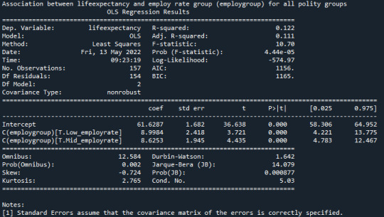
“P-value = 4.44e-05, the null hypothesis is rejected and can be concluded that the life expectancy is dependent on the employ group.”

Is there an association between life expectancy and employ rate group (employgroup) in those countries with Low_polityscore (polityscore)?:

model2 = smf.ols(formula='lifeexpectancy ~ C(employgroup)', data=sub6)

results2 = model2.fit()

print (results2.summary())

“P-value = 0.120, the null hypothesis cannot be rejected and life expectancy is not dependent on employ rate for countries with low_polityscore”

Is there an association between lifeexpectancy and employ rate group (employgroup) in those countries with Mid_polityscore (polityscore)?:

model3 = smf.ols(formula='lifeexpectancy ~ C(employgroup)', data=sub7)

results3 = model3.fit()

print (results3.summary())

"P-value = 0.00582, null hypothesis can be rejected and life expectancy is dependent on employ rate for countries with mid_polityscore.”

Is there an association between lifeexpectancy and employ rate group (employgroup) in those countries with High_polityscore (polityscore)?:

model4 = smf.ols(formula='lifeexpectancy ~ C(employgroup)', data=sub8)

results4 = model4.fit()

print (results4.summary())

“P-value = 0.0022 null hypothesis can be rejected and life expectancy is dependent on employ rate for countries with high_polityscore.”

0 notes

rocio-engineer-blog · 2 years

Text

Data Analysis Tools Week 3

Generating a Correlation Coefficient

Generate a correlation coefficient.

Note 1: Two 3+ level categorical variables can be used to generate a correlation coefficient if the the categories are ordered and the average (i.e. mean) can be interpreted. The scatter plot on the other hand will not be useful. In general the scatterplot is not useful for discrete variables (i.e. those that take on a limited number of values).

Note 2: When we square r, it tells us what proportion of the variability in one variable is described by variation in the second variable (a.k.a. RSquared or Coefficient of Determination)

Continuing with the previous assigment, we will run 2 Pearson correlation test to see:

Is there a correlation between Urban rate and Internet use rate?

2. Is there a correlation between Income per person and internet use rate?

Code and results:

import numpy

import pandas

import statsmodels.formula.api as smf

import statsmodels.stats.multicomp as multi

import scipy.stats

import seaborn

import matplotlib.pyplot as plt

# Load gapminder dataset

data = pandas.read_csv(’_7548339a20b4e1d06571333baf47b8df_gapminder.csv’, low_memory=False)

# To avoid having blank data instead of NaN -> If you have blank data the previous line will give you an error.

data = data.replace(r’^\s*$’, numpy.NaN, regex = True)

# Change all DataFrame column names to Lower-case

data.columns = map(str.lower, data.columns)

# Bug fix for display formats to avoid run time errors

pandas.set_option(‘display.float_format’, lambda x:’%f’%x)

print('Number of observations (rows)’)

print(len(data))

print('Number of Variables (columns)’)

print(len(data.columns))

print()

# Ensure each of these columns are numeric

data['suicideper100th’] = data['suicideper100th’].apply(pandas.to_numeric, errors='coerce’)

data['lifeexpectancy’] = data['lifeexpectancy’].apply(pandas.to_numeric, errors='coerce’)

data['urbanrate’] = data['urbanrate’].apply(pandas.to_numeric, errors='coerce’)

data['employrate’] = data['employrate’].apply(pandas.to_numeric, errors='coerce’)

data['polityscore’] = data['polityscore’].apply(pandas.to_numeric, errors='coerce’)

data['internetuserate’] = data['internetuserate’].apply(pandas.to_numeric, errors='coerce’)

data['incomeperperson’] = data['incomeperperson’].apply(pandas.to_numeric, errors='coerce’)

# Pearson correlation:

# Pearson Correlation Coefficient r: Measures a linear relationship between 2 quantitative variables (Quantitative relational variable and quantitative response variable)

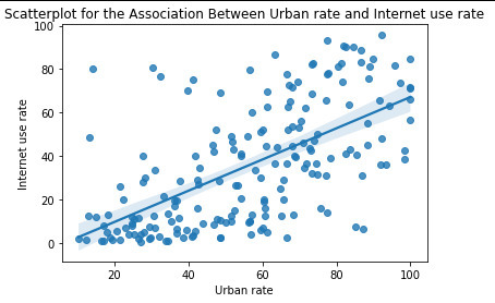
-Is there a correlation between Urban rate and Internet use rate?

scat1 = seaborn.regplot(x= 'urbanrate’, y= 'internetuserate’, fit_reg=True, data=data)

plt.xlabel('Urban rate’)

plt.ylabel('Internet use rate’)

plt.title('Scatterplot for the Association Between Urban rate and Internet use rate’)

print('Association between urbanrate and internetuserate’)

print('Correlation coeficient, p-value’)

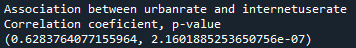
The relationship is positive with a significan p-value, hence having a high urban rate leads to a high internet use

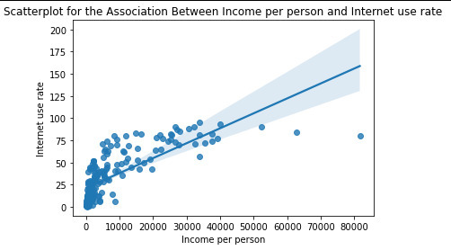
-Is there a correlation between Income per person and internet use rate?

scat2 = seaborn.regplot(x= 'incomeperperson’, y= 'internetuserate’, fit_reg=True, data=data)

plt.xlabel('Income per person’)

plt.ylabel('Internet use rate’)

plt.title('Scatterplot for the Association Between Income per person and Internet use rate’)

data_cleaned = data.dropna()

print('Association between incomeperperson and internetuserate’)

print('Correlation coeficient, p-value’)

The relationship is positive with a significan p-value, hence having a high income per person leads to a high internet use.

0 notes

rocio-engineer-blog · 2 years

Text

Week 2 Data Management & Visualization

Chi Square Test of Independency Assigment

Instructions:

Run a Chi-Square Test of Independence.

You will need to analyze and interpret post hoc paired comparisons in instances where your original statistical test was significant, and you were examining more than two groups (i.e. more than two levels of a categorical, explanatory variable).

Note: although it is possible to run large Chi-Square tables (e.g. 5 x 5, 4 x 6, etc.), the test is really only interpretable when your response variable has only 2 levels (see Graphing decisions flow chart in Bivariate Graphing chapter).

Submission:

By continuing with the previous week homework, we will run 2 chi-square test to try to see:

-‘Do polity score depends on the country group type?’ (PIGS vs EasternEurope vs Rest)

-For all countries, do the polity score of a country affect its employ rate?

Code and results:

import numpy import pandas import statsmodels.formula.api as smf import statsmodels.stats.multicomp as multi import scipy.stats

# Load gapminder dataset data = pandas.read_csv(’_7548339a20b4e1d06571333baf47b8df_gapminder.csv’, low_memory=False)

# To avoid having blank data instead of NaN -> If you have blank data the previous line will give you an error. data = data.replace(r’^\s*$’, numpy.NaN, regex = True)

# Change all DataFrame column names to Lower-case data.columns = map(str.lower, data.columns)

# Bug fix for display formats to avoid run time errors pandas.set_option('display.float_format’, lambda x:’%f’%x)

print('Number of observations (rows)’) print(len(data)) print('Number of Variables (columns)’) print(len(data.columns)) print()

# Ensure each of these columns are numeric data['suicideper100th’] = data['suicideper100th’].apply(pandas.to_numeric, errors='coerce’) data['lifeexpectancy’] = data['lifeexpectancy’].apply(pandas.to_numeric, errors='coerce’) data['urbanrate’] = data['urbanrate’].apply(pandas.to_numeric, errors='coerce’) data['employrate’] = data['employrate’].apply(pandas.to_numeric, errors='coerce’) data['polityscore’] = data['polityscore’].apply(pandas.to_numeric, errors='coerce’) print(data['polityscore’])

# Filtering into groups: print('According to the definition below for Easter European countries and PIGS countries we will create a new column called EuropeEastVsPIGS where:’) print('1 is for Eastern Europe: Bulgaria, Czech Rep., Hungary, Poland, Romania, Russian Federation, Slovakia, Belarus, Moldova and Ukraine’) print('2 is for PiGS countries: Portual, Ireland, Italy, Greece and Spain ’) print()

def EuropeEastVsPIGS (row) : if row['country’] == 'Bulgaria’: return 1 if row['country’] == 'Czech Rep.’: return 1 if row['country’] == 'Hungary’: return 1 if row['country’] == 'Poland’: return 1 if row['country’] == 'Romania’: return 1 if row['country’] == 'Russia’: return 1 if row['country’] == 'Slovak Republic’: return 1 if row['country’] == 'Belarus’: return 1 if row['country’] == 'Moldova’: return 1 if row['country’] == 'Ukraine’: return 1 if row['country’] == 'Portugal’: return 2 if row['country’] == 'Ireland’: return 2 if row['country’] == 'Italy’: return 2 if row['country’] == 'Greece’: return 2 if row['country’] == 'Spain’: return 2

data['EuropeEastVsPIGS’] = data.apply (lambda row: EuropeEastVsPIGS (row), axis = 1) data['EuropeEastVsPIGS’] = data['EuropeEastVsPIGS’].apply(pandas.to_numeric, errors='coerce’)

# Replace NaN with 99 to use as others data['EuropeEastVsPIGS’].fillna(99, inplace=True)

sub1 = data.copy()

# Chi Square test of independence: when we have a categorical explanatory variabale and a categorial response variable:

-'Do polity score depends on the country group type?’ # Convert a cuantitative variable into a categorical: We will group the polityscore intro 4 cathegories:

def politygroup (row) : if row['polityscore’] >= -10 and row['polityscore’] < -3 : return 'NegativePolity’ if row['polityscore’] >= -3 and row['polityscore’] < 4 : return 'NeutralPolity’ if row['polityscore’] >= 4 and row['polityscore’] < 11 : return 'PositivePolity’

sub1['politygroup’] = sub1.apply (lambda row: politygroup (row), axis = 1)

sub4 = sub1[['EuropeEastVsPIGS’,'politygroup’]].dropna()

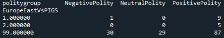
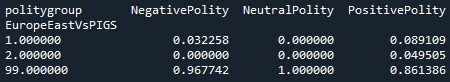
Since the p-value = 0.134 we cannot reject the null hypothesis and hence there are no diferences between the groups defined. The results are based on having a “Rest of the world” group that has a lot of countries on it.

-For all countries, do the polity score of a country affect its employ rate?

# Another example of the use of Chi-Square: print('For all countries, do polity score group affect the employ rate of a country?’)

sub5 = sub1[['politygroup’,'employrate’]].dropna()

# Group into 3 categories the employ rate of countries # Change NaN values to 0 to get max value in employ rate column sub6 = sub5.copy() sub6.fillna(0, inplace=True) sub6_maxer = sub6['employrate’].max()

sub7 = sub5.copy() sub7.fillna(999, inplace=True) sub7_min = sub7['employrate’].min()

employlow = 0.33*(sub6_maxer - sub7_min) + sub7_min employhigh = 0.66*(sub6_maxer - sub7_min) + sub7_min

def employgroup (row) : if row['employrate’] >= sub7_min and row['employrate’] < employlow : return 'Low_employrate’ if row['employrate’] >= employlow and row['employrate’] < employhigh : return 'Mid_employrate’ if row['employrate’] >= employhigh and row['employrate’] <= sub6_maxer : return 'High_employrate’

sub5['employgroup’] = sub1.apply (lambda row: employgroup (row), axis = 1)

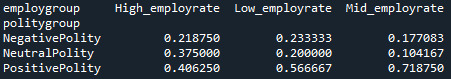
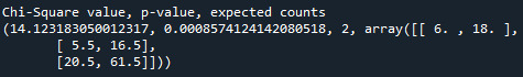
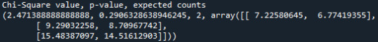
Since the p-value = 0.0059, null hypothesis is rejected and we can conclude that the employ rate depends on the polityscore of the country. We know they are not equal but we dont know which ones are equals and which are not. To know this a post-hoc test is needed.

# If we reject the null hypothesis, we need to perform comparisons for each pair of groups. # To appropiate protect against type 1 error in the contxt of a chi-squared test, we wil use the post-hoc called “Bonferroni Adjustment”

# For that we will make 2 groups comparisons:

# For 1st pair of groups:

recode3 = {'High_employrate’:'High_employrate’ , 'Mid_employrate’:'Mid_employrate’ } sub5['Comp1vs2’] = sub5['employgroup’].map(recode3)

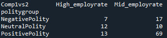
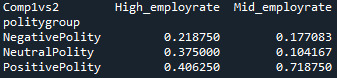
Since the p-value = 0.00086, null hypothesis is rejected and we can conclude that there is a significant difference between this 2 groups. High_employrate group is different from Mid_employrate group.

# For 2nd pair of groups:

recode4 = {'High_employrate’:'High_employrate’ , 'Low_employrate’:'Low_employrate’ } sub5['Comp1vs3’] = sub5['employgroup’].map(recode4)

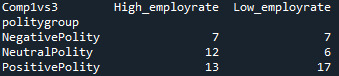
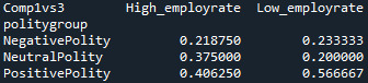
Since the p-value = 0.29063, null hypothesis cannot be rejected and we can conclude that there is no significant difference between this 2 groups. High_employrate group is simmilar to low_employ rate group.

# For 3rd pair of groups:

recode5 = {'Low_employrate’:'Low_employrate’ , 'Mid_employrate’:'Mid_employrate’ } sub5['Comp2vs3’] = sub5['employgroup’].map(recode5)

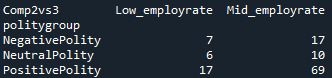
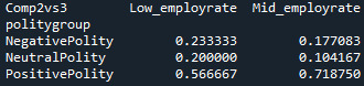
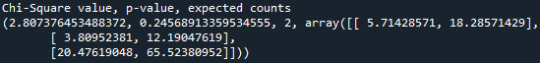
Since the p-value = 0.24568, null hypothesis cannot be rejected and we can conclude that there is no significant difference between this 2 groups. Mid_employrate group is simmilar to low_employ rate group.

0 notes

rocio-engineer-blog · 2 years

Text

Week 4: Creating graphs for your data

By continuing with the previous week homework, we will run an ANOVA analysis that includes a moderator to try to see:

-Life expectancy of a country depends on its employ rate?

-Is the polity score of the country a good moderator?

Code and results of running it:

# -*- coding: utf-8 -*- """ Created on Tue Apr 19 16:42:34 202

"""

import numpy import pandas import statsmodels.formula.api as smf import statsmodels.stats.multicomp as multi import scipy.stats import seaborn import matplotlib.pyplot as plt

# Load gapminder dataset

data = pandas.read_csv('_7548339a20b4e1d06571333baf47b8df_gapminder.csv', low_memory=False)

# To avoid having blank data instead of NaN -> If you have blank data the previous line will give you an error.

data = data.replace(r'^\s*$', numpy.NaN, regex = True)

# Change all DataFrame column names to Lower-case

data.columns = map(str.lower, data.columns)

# Bug fix for display formats to avoid run time errors

pandas.set_option('display.float_format', lambda x:'%f'%x)

print('Number of observations (rows)') print(len(data)) print('Number of Variables (columns)') print(len(data.columns)) print()

# Ensure each of these columns are numeric

data['suicideper100th'] = data['suicideper100th'].apply(pandas.to_numeric, errors='coerce') data['lifeexpectancy'] = data['lifeexpectancy'].apply(pandas.to_numeric, errors='coerce') data['urbanrate'] = data['urbanrate'].apply(pandas.to_numeric, errors='coerce') data['employrate'] = data['employrate'].apply(pandas.to_numeric, errors='coerce') data['polityscore'] = data['polityscore'].apply(pandas.to_numeric, errors='coerce') data['internetuserate'] = data['internetuserate'].apply(pandas.to_numeric, errors='coerce') data['incomeperperson'] = data['incomeperperson'].apply(pandas.to_numeric, errors='coerce')

# Convert a cuantitative variable into a categorical: We will group the polityscore intro 3 cathegories:

def politygroup (row) : if row['polityscore'] >= -10 and row['polityscore'] < -3 : return 'NegativePolity' if row['polityscore'] >= -3 and row['polityscore'] < 4 : return 'NeutralPolity' if row['polityscore'] >= 4 and row['polityscore'] < 11 : return 'PositivePolity'

sub1['politygroup'] = sub1.apply (lambda row: politygroup (row), axis = 1)

sub5 = sub1[['politygroup','employrate','suicideper100th','lifeexpectancy']].dropna()

# Moderator: A third variable that affects the direction and/or strength of the relation between your explanatory or x variable and your response or y variable

# Testing a moderator in the context of ANOVA:

Let’s evaluate if suicide rate Employ rate groups (Low, Mid and Hihg employ rates), Polity score groups (Negative, Neutral and Positive polity scores):

sub6 = sub5[(sub5['politygroup'] == 'NegativePolity')] sub7 = sub5[(sub5['politygroup'] == 'NeutralPolity')] sub8 = sub5[(sub5['politygroup'] == 'PositivePolity')]

print('Association between lifeexpectancy and employ rate group (employgroup) for all polity groups') model99 = smf.ols(formula='lifeexpectancy ~ C(employgroup)', data=sub5) results99 = model99.fit() print (results99.summary())

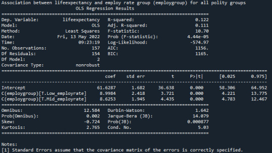
“Since p-value = 4.44e-05 so null hypothesis is rejected and we conclude that the life expectancy is dependent on the employ group.”

Is there an association between lifeexpectancy and employ rate group (employgroup) in those countries with Low_polityscore (polityscore)?:

model2 = smf.ols(formula='lifeexpectancy ~ C(employgroup)', data=sub6) results2 = model2.fit() print (results2.summary())

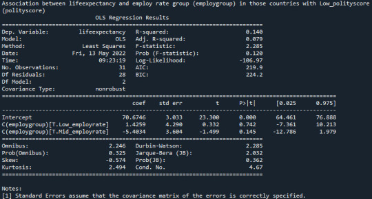
“Since p-value = 0.120 so null hypothesis cannot be rejected and life expectancy is not dependent on employ rate for countries with low_polityscore”

Is there an association between lifeexpectancy and employ rate group (employgroup) in those countries with Mid_polityscore (polityscore)?:

model3 = smf.ols(formula='lifeexpectancy ~ C(employgroup)', data=sub7) results3 = model3.fit() print (results3.summary())

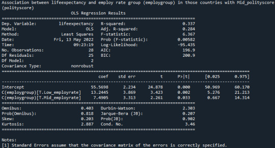
"Since p-value = 0.00582 null hypothesis can be rejected and life expectancy is dependent on employ rate for countries with mid_polityscore.”

Is there an association between lifeexpectancy and employ rate group (employgroup) in those countries with High_polityscore (polityscore)?: model4 = smf.ols(formula='lifeexpectancy ~ C(employgroup)', data=sub8) results4 = model4.fit() print (results4.summary())

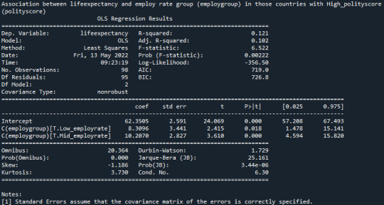
“Since p-value = 0.0022 null hypothesis can be rejected and life expectancy is dependent on employ rate for countries with high_polityscore.”

1 note · View note

rocio-engineer-blog · 2 years

Text

Week 3: Data Management

Program

# Import python libraries for data management import pandas as pd import numpy

# Load in CSV file data = pd.read_csv('ool_pds.csv', low_memory=False)

# Print numbers of rows and columns print("Number of observations or rows") print(len(data)) # Number of observations or rows print("Number of variables or columns") print(len(data.columns)) # Number of variables or columns

# Ensure data types are numeric print("Data types of variables") print("Data type of PPGENDER for gender") print(data['PPGENDER'].dtypes) print("Data type of PPINCIMP for household income") print(data['PPINCIMP'].dtypes) print("Data type of W1_B1 for government empathy for identity group") print(data['W1_B1'].dtypes)

# Frequency distribution of gender assigned to c1. Find variable in data frame. print("Gender count, 1 = male, 2 = female") c1 = data["PPGENDER"].value_counts(sort=False, dropna=False) print (c1)

print("Gender percent, 1 = male, 2 = female") # Normalize parameter describes percentage p1 = data["PPGENDER"].value_counts(sort=False, normalize=True) print(p1)

print("Household Income count, 1 = less than 50k, ascending") c2 = data["PPINCIMP"].value_counts(sort=False, dropna=False) print(c2)

print("Household Income percent, 1 = less than 50k, ascending") p2 = data["PPINCIMP"].value_counts(sort=False, normalize=True) print(p2)

print("Government empathy for identity group count, 1 = great deal, descending") c3 = data["W1_B1"].value_counts(sort=False, dropna=False) print(c3)

print("Government empathy for identity group percent, 1 = great deal, descending") p3 = data["W1_B1"].value_counts(sort=False, normalize=True) print(p3)

# Create a subset of data to manage missing values sub1=data.copy()

# Replace "Refused" response with Nan value sub1['W1_B1']=sub1['W1_B1'].replace(-1, numpy.nan)

# Check to ensure that NaN values are removed print("Government empathy for identity group count, 1 = great deal, descending") c4 = sub1["W1_B1"].value_counts(sort=False, dropna=False) print(c4)

# Recodes measure of Government Empathy for "5" to represent "a great deal" recode1 = {1: 5, 2: 4, 3: 3, 4: 2, 5: 1} sub1['GOVEMP']= sub1['W1_B1'].map(recode1)

# Check for successful recoding print("Government empathy for identity group count, 1 = not at all, descending") c5 = sub1['GOVEMP'].value_counts(sort=False, dropna=False) print(c5)

# Recodes income by quantitative income measure defined by max income of bucket recode2 = {1: 5000, 2: 7499, 3: 9999, 4: 12499, 5: 14999, 6: 19999, 7: 24999, 8: 29999, 9: 34999, 10: 39999, 11: 49999, 12: 59999, 13: 74999, 14: 84999, 15: 99999, 16: 124999, 17: 149999, 18: 174999, 19: 175000} sub1['INCOME']= sub1['PPINCIMP'].map(recode2)

# Check for succesful recording print("Household Income count by bin indicating max in bucket") c6 = sub1['INCOME'].value_counts(sort=False, dropna=False) print(c6)

# Redistributed succinct income buckets in 25k buckets starting with 5000 minimum household income sub1['INCOMECUT']=pd.cut(sub1.INCOME, [0, 24999, 49999, 74999, 99999, 124999, 149999, 174999, 175000])

print("Household Income count by 25k buckets") c8 = sub1['INCOMECUT'].value_counts(sort=False, dropna=True) print(c8)

print("Household Income percent by 25k buckets") p8 = sub1['INCOMECUT'].value_counts(sort=False, dropna=True, normalize= True) print(p8)

# Check for correct grouping of income print(pd.crosstab(sub1['INCOMECUT'],sub1['INCOME']))

Output

Number of observations or rows 2294 Number of variables or columns 436 Data types of variables Data type of PPGENDER for gender int64 Data type of PPINCIMP for household income int64 Data type of W1_B1 for government empathy for identity group int64 Gender count, 1 = male, 2 = female 2 1262 1 1032 Name: PPGENDER, dtype: int64 Gender percent, 1 = male, 2 = female 2 0.550131 1 0.449869 Name: PPGENDER, dtype: float64 Household Income count, 1 = less than 50k, ascending

2 64 4 68 6 98 8 140 10 132 12 181 14 129 16 200 18 63 1 127 3 61 5 62 7 109 9 108 11 162 13 235 15 145 17 125 19 85

Name: PPINCIMP, dtype: int64 Household Income percent, 1 = less than 50k, ascending 2 0.027899 4 0.029643 6 0.042720 8 0.061029 10 0.057541 12 0.078901 14 0.056234 16 0.087184 18 0.027463 1 0.055362 3 0.026591 5 0.027027 7 0.047515 9 0.047079 11 0.070619 13 0.102441 15 0.063208 17 0.054490 19 0.037053

Name: PPINCIMP, dtype: float64 Government empathy for identity group count, 1 = great deal, descending 2 203 4 780 -1 24 1 83 3 672 5 532 Name: W1_B1, dtype: int64 Government empathy for identity group percent, 1 = great deal, descending 2 0.088492 4 0.340017 -1 0.010462 1 0.036181 3 0.292938 5 0.231909 Name: W1_B1, dtype: float64 Government empathy for identity group count, 1 = great deal, descending NaN 24 1 83 2 203 3 672 4 780 5 532 Name: W1_B1, dtype: int64 Government empathy for identity group count, 1 = not at all, descending NaN 24 1 532 2 780 3 672 4 203 5 83 Name: GOVEMP, dtype: int64 Household Income count by bin indicating max in bucket 124999 200 34999 108 149999 125 59999 181 14999 62 5000 127 174999 63 84999 129 39999 132 7499 64 19999 98 12499 68 24999 109 49999 162 175000 85 74999 235 29999 140 99999 145 9999 61

Name: INCOME, dtype: int64 Household Income count by 25k buckets

(0, 24999] 589 (24999, 49999] 542 (49999, 74999] 416 (74999, 99999] 274 (99999, 124999] 200 (124999, 149999] 125 (149999, 174999] 63 (174999, 175000] 85

dtype: int64 Household Income percent by 25k buckets (0, 24999] 0.256757 (24999, 49999] 0.236269 (49999, 74999] 0.181343 (74999, 99999] 0.119442 (99999, 124999] 0.087184 (124999, 149999] 0.054490 (149999, 174999] 0.027463 (174999, 175000] 0.037053 dtype: float64 INCOME 5000 7499 9999 12499 14999 19999 24999 \

INCOMECUT (0, 24999] 127 64 61 68 62 98 109 (24999, 49999] 0 0 0 0 0 0 0 (49999, 74999] 0 0 0 0 0 0 0 (74999, 99999] 0 0 0 0 0 0 0 (99999, 124999] 0 0 0 0 0 0 0 (124999, 149999] 0 0 0 0 0 0 0 (149999, 174999] 0 0 0 0 0 0 0 (174999, 175000] 0 0 0 0 0 0 0

NCOME 99999 124999 149999 174999 175000 INCOMECUT (0, 24999] 0 0 0 0 0 (24999, 49999] 0 0 0 0 0 (49999, 74999] 0 0 0 0 0 (74999, 99999] 145 0 0 0 0 (99999, 124999] 0 200 0 0 0 (124999, 149999] 0 0 125 0 0 (149999, 174999] 0 0 0 63 0 (174999, 175000] 0 0 0 0 85

Last Week Summary Review

My data set has 2294 observations/ rows and 436 variables/ observations. Of these variables, I chose three for which to display frequency tables including gender, household income, and a variable I’m calling, “government empathy for identity group”. According to my results, 55% of the respondents are female and 44% are male. Of the 19 buckets for household income spanning from less than $5,000 to $175,000 or more, $60,000 - $74,999 is the most frequent household income bracket reported at 10%. In response to the question, “How much do government officials care about what people like you think?” or my government empathy variable, 34% of respondents reported “A little”. The responses ranged from “A Great Deal” encoded in 1 to “Not at all” encoded in five.

There were no missing values in this data set because refusal to answer was captured by “-1″, which can be excluded.

This Week Summary

Of my three variables, I recoded two this week to make my data more manageable and straightforward:

Gender - No recode necessary, binary values for male vs. female

Government Empathy for Identity Group - Recoded so that a measure of “5″, the highest measure, would indicate “A Great Deal” and “1″ would be “Not at All” instead of the opposite. This makes more sense logically. In addition, I removed the presence of “Refused” answers by setting them equal to Nan.

Household Income - Recoded so that instead of measures of 1-19, I changed it to indicate the maximum income of that bucket. For example, a measure of 5000 would indicate that those respondents had a maximum of $5,000 in household income. In addition, I had to do further work to make this data useful because not all the buckets were the same size. Some were $2,500, others were $5,000 and it changed all the way up to $25,000. For example, value 2 indicated a bucket of between $5,000 and $7,499 in household income, a bucket of $2,499 and value 16 indicated household income between $100,000 and $124,999, a difference of $24,999.

The biggest change in my variables this week was the way I summarized “Household Income”. Now I can see that the greatest percentage of respondents, about 25%, had income of $24,999 or less, followed by about 23% of respondents having an income of $49,999 or less. Between these two groups, almost 50% of respondents had an income of $49,999 or less. Another interesting observation is that more respondents, about 3.7% or 85 respondents, had incomes of $175k+, which is greater than the number of respondents in the adjacent lower bucket of $150,000 - $174,999.

0 notes

rocio-engineer-blog · 2 years

Text

Week 2: Python Program and Frequency Distributions

Program:

# Import python libraries for data management import pandas as pd import numpy

# Load in CSV file data = pd.read_csv('ool_pds.csv', low_memory=False)

# Print numbers of rows and columns print(len(data)) # Number of observations or rows print(len(data.columns)) # Number of variables or columns

# Ensure data types are numeric print(data['PPGENDER'].dtypes) print(data['PPINCIMP'].dtypes) print(data['W1_B1'].dtypes)

# Frequency distribution of gender assigned to c1. Find variable in data frame. print("Gender count, 1 = male, 2 = female") c1 = data["PPGENDER"].value_counts(sort=False, dropna=False) print (c1)

print("Gender percent, 1 = male, 2 = female") # Normalize parameter describes percentage p1 = data["PPGENDER"].value_counts(sort=False, normalize=True) print(p1)

print("Household Income count, 1 = less than 50k, ascending") c2 = data["PPINCIMP"].value_counts(sort=False, dropna=False) print(c2)

print("Household Income percent, 1 = less than 50k, ascending") p2 = data["PPINCIMP"].value_counts(sort=False, normalize=True) print(p2)

print("Government empathy for identity group count, 1 = great deal, descending") c3 = data["W1_B1"].value_counts(sort=False, dropna=False) print(c3)

print("Government empathy for identity group percent, 1 = great deal, descending") p3 = data["W1_B1"].value_counts(sort=False, normalize=True) print(p3)

# Subset data to display only relevant values. In this case, removing refused answer for W1_B1

sub1=data[(data['W1_B1']>0)]

# Makes a copy of the subset of data sub2=sub1.copy()

Output:

Number of observations or rows 2294 Number of variblaes or columns 436 Data types of variables Data type of PPGENDER for gender int64 Data type of PPINCIMP for household income int64 Data type of W1_B1 for government empathy for identity group int64 Gender count, 1 = male, 2 = female 2 1262 1 1032 Name: PPGENDER, dtype: int64 Gender percent, 1 = male, 2 = female 2 0.550131 1 0.449869 Name: PPGENDER, dtype: float64 Household Income count, 1 = less than 50k, ascending 2 64 4 68 6 98 8 140 10 132 12 181 14 129 16 200 18 63 1 127 3 61 5 62 7 109 9 108 11 162 13 235 15 145 17 125 19 85 Name: PPINCIMP, dtype: int64 Household Income percent, 1 = less than 50k, ascending 2 0.027899 4 0.029643 6 0.042720 8 0.061029 10 0.057541 12 0.078901 14 0.056234 16 0.087184 18 0.027463 1 0.055362 3 0.026591 5 0.027027 7 0.047515 9 0.047079 11 0.070619 13 0.102441 15 0.063208 17 0.054490 19 0.037053 Name: PPINCIMP, dtype: float64 Government empathy for identity group count, 1 = great deal, descending 2 203 4 780 -1 24 1 83 3 672 5 532 Name: W1_B1, dtype: int64 Government empathy for identity group percent, 1 = great deal, descending 2 0.088492 4 0.340017 -1 0.010462 1 0.036181 3 0.292938 5 0.231909 Name: W1_B1, dtype: float64

Summary:

Data set has 2294 observations/ rows and 436 variables/ observations. Of these variables, I chose three for which to display frequency tables including gender, household income, and a variable I’m calling, “government empathy for identity group”. According to my results, 55% of the respondents are female and 44% are male. Of the 19 buckets for household income spanning from less than $5,000 to $175,000 or more, $60,000 - $74,999 is the most frequent household income bracket reported at 10%. In response to the question, “How much do government officials care about what people like you think?” or my government empathy variable, 34% of respondents reported “A little”. The responses ranged from “A Great Deal” encoded in 1 to “Not at all” encoded in five.

There were no missing values in this data set because refusal to answer was captured by “-1″, which can be excluded.

0 notes