research-regression

[research-regression]

Logistic Regression Model

Hypothesis: The rate of Alcohol consumption and/or the level of income may influence the probability of commiting a suicide.

Results: After adjusting for potential confounding factors (Gross Domestic Product per capita in constant 2000 US$, Alcohol Consumption Rate), the odds of commiting a suicide were higher for countries where people consume more alcohol (OR=1.14, 95% CI = 1.07-1.22, p=.0001). However, the income was not significantly associated with suicide (OR= 1.00, 95% CI=1.00-1.00, p=.292). No confounding variables were indicated.

Code:

import pandas as pd import numpy as np import statsmodels.api as sm import statsmodels.formula.api as smf import seaborn import matplotlib.pyplot as plt pd.set_option('display.float_format', lambda x:'%.2f'%x) data = pd.read_csv('gapminder.csv') data['suicideper100th'] = pd.to_numeric(data['suicideper100th'], errors='coerce') data['alcconsumption'] = pd.to_numeric(data['alcconsumption'], errors='coerce') data['incomeperperson'] = pd.to_numeric(data['incomeperperson'], errors='coerce') sub1 = data[['alcconsumption', 'suicideper100th', 'incomeperperson']].dropna() sub1['alcconsumption_c'] = (sub1['alcconsumption'] - sub1['alcconsumption'].mean()) sub1['incomeperperson_c'] = (sub1['incomeperperson'] - sub1['incomeperperson'].mean()) sub1["suicideper100th"] = sub1["suicideper100th"].apply(lambda x: 0 if x < sub1['suicideper100th'].mean() else 1) print(sub1[["alcconsumption_c", "incomeperperson_c", "suicideper100th"]].describe()) lreg1 = smf.logit(formula = 'suicideper100th ~ alcconsumption_c', data = sub1).fit() print (lreg1.summary()) # odds ratios print ("Odds Ratios") print (np.exp(lreg1.params)) params = lreg1.params conf = lreg1.conf_int() conf['OR'] = params conf.columns = ['Lower CI', 'Upper CI', 'OR'] print (np.exp(conf)) lreg1 = smf.logit(formula = 'suicideper100th ~ incomeperperson_c', data = sub1).fit() print (lreg1.summary()) # odds ratios print ("Odds Ratios") print (np.exp(lreg1.params)) params = lreg1.params conf = lreg1.conf_int() conf['OR'] = params conf.columns = ['Lower CI', 'Upper CI', 'OR'] print (np.exp(conf)) lreg2 = smf.logit(formula = 'suicideper100th ~ alcconsumption_c + incomeperperson_c', data = sub1).fit() print (lreg2.summary()) params = lreg2.params conf = lreg2.conf_int() conf['OR'] = params conf.columns = ['Lower CI', 'Upper CI', 'OR'] print (np.exp(conf))

Output:

alcconsumption_c incomeperperson_c suicideper100th count 177.00 177.00 177.00 mean 0.00 -0.00 0.44 std 4.91 10166.20 0.50 min -6.79 -6984.62 0.00 25% -4.08 -6374.75 0.00 50% -0.72 -4662.92 0.00 75% 3.15 1357.13 1.00 max 16.17 45213.19 1.00 Optimization terminated successfully. Current function value: 0.637312 Iterations 5 Logit Regression Results ============================================================================== Dep. Variable: suicideper100th No. Observations: 177 Model: Logit Df Residuals: 175 Method: MLE Df Model: 1 Date: Sun, 13 Mar 2022 Pseudo R-squ.: 0.06918 Time: 18:17:57 Log-Likelihood: -112.80 converged: True LL-Null: -121.19 Covariance Type: nonrobust LLR p-value: 4.223e-05 ==================================================================================== coef std err z P>|z| [0.025 0.975] ------------------------------------------------------------------------------------ Intercept -0.2761 0.159 -1.734 0.083 -0.588 0.036 alcconsumption_c 0.1334 0.034 3.872 0.000 0.066 0.201 ==================================================================================== Odds Ratios Intercept 0.76 alcconsumption_c 1.14 dtype: float64 Lower CI Upper CI OR Intercept 0.56 1.04 0.76 alcconsumption_c 1.07 1.22 1.14 Optimization terminated successfully. Current function value: 0.681521 Iterations 4 Logit Regression Results ============================================================================== Dep. Variable: suicideper100th No. Observations: 177 Model: Logit Df Residuals: 175 Method: MLE Df Model: 1 Date: Sun, 13 Mar 2022 Pseudo R-squ.: 0.004615 Time: 18:17:57 Log-Likelihood: -120.63 converged: True LL-Null: -121.19 Covariance Type: nonrobust LLR p-value: 0.2902 ===================================================================================== coef std err z P>|z| [0.025 0.975] ------------------------------------------------------------------------------------- Intercept -0.2624 0.152 -1.725 0.085 -0.560 0.036 incomeperperson_c 1.576e-05 1.5e-05 1.054 0.292 -1.35e-05 4.51e-05 ===================================================================================== Odds Ratios Intercept 0.77 incomeperperson_c 1.00 dtype: float64 Lower CI Upper CI OR Intercept 0.57 1.04 0.77 incomeperperson_c 1.00 1.00 1.00 Optimization terminated successfully. Current function value: 0.637215 Iterations 5 Logit Regression Results ============================================================================== Dep. Variable: suicideper100th No. Observations: 177 Model: Logit Df Residuals: 174 Method: MLE Df Model: 2 Date: Sun, 13 Mar 2022 Pseudo R-squ.: 0.06932 Time: 18:17:57 Log-Likelihood: -112.79 converged: True LL-Null: -121.19 Covariance Type: nonrobust LLR p-value: 0.0002246 ===================================================================================== coef std err z P>|z| [0.025 0.975] ------------------------------------------------------------------------------------- Intercept -0.2756 0.159 -1.731 0.083 -0.588 0.036 alcconsumption_c 0.1355 0.036 3.721 0.000 0.064 0.207 incomeperperson_c -3.011e-06 1.62e-05 -0.185 0.853 -3.48e-05 2.88e-05 ===================================================================================== Lower CI Upper CI OR Intercept 0.56 1.04 0.76 alcconsumption_c 1.07 1.23 1.15 incomeperperson_c 1.00 1.00 1.00

[research-regression]

Multiple Regression Model

Hypothesis: Gross Domestic Product per capita in constant 2000 US$ may confound the relationship between Alcohol Consumption Rate and Suicide Rate.

Results: After adjusting for potential confounding factors (Gross Domestic Product per capita in constant 2000 US$), Alcohol Consumption Rate (Beta=0.5274, p=.0001) was significantly and positively associated with Suicide Rate. Gross Domestic Product per capita in constant 2000 US$ (Beta=-7.114e-05, p=.11) was not associated with Suicide Rate.

Code:

import pandas as pd import numpy as np import statsmodels.api as sm import statsmodels.formula.api as smf import seaborn import matplotlib.pyplot as plt pd.set_option('display.float_format', lambda x:'%.2f'%x) data = pd.read_csv('gapminder.csv') data['suicideper100th'] = pd.to_numeric(data['suicideper100th'], errors='coerce') data['alcconsumption'] = pd.to_numeric(data['alcconsumption'], errors='coerce') data['incomeperperson'] = pd.to_numeric(data['incomeperperson'], errors='coerce') sub1 = data[['alcconsumption', 'suicideper100th', 'incomeperperson']].dropna() sub1['alcconsumption_c'] = (sub1['alcconsumption'] - sub1['alcconsumption'].mean()) sub1['incomeperperson_c'] = (sub1['incomeperperson'] - sub1['incomeperperson'].mean()) sub1[["alcconsumption_c", "incomeperperson_c"]].describe() reg2 = smf.ols('suicideper100th ~ alcconsumption_c + incomeperperson_c', data=sub1).fit() print (reg2.summary()) `</pre><pre>` OLS Regression Results ============================================================================== Dep. Variable: suicideper100th R-squared: 0.160 Model: OLS Adj. R-squared: 0.150 Method: Least Squares F-statistic: 16.59 Date: Sat, 12 Mar 2022 Prob (F-statistic): 2.54e-07 Time: 15:48:25 Log-Likelihood: -557.80 No. Observations: 177 AIC: 1122. Df Residuals: 174 BIC: 1131. Df Model: 2 Covariance Type: nonrobust ===================================================================================== coef std err t P>|t| [0.025 0.975] ------------------------------------------------------------------------------------- Intercept 9.6275 0.429 22.459 0.000 8.781 10.474 alcconsumption_c 0.5274 0.092 5.760 0.000 0.347 0.708 incomeperperson_c -7.114e-05 4.42e-05 -1.609 0.110 -0.000 1.62e-05 ============================================================================== Omnibus: 47.034 Durbin-Watson: 2.060 Prob(Omnibus): 0.000 Jarque-Bera (JB): 97.970 Skew: 1.216 Prob(JB): 5.32e-22 Kurtosis: 5.715 Cond. No. 1.01e+04 ============================================================================== Notes: [1] Standard Errors assume that the covariance matrix of the errors is correctly specified. [2] The condition number is large, 1.01e+04. This might indicate that there are strong multicollinearity or other numerical problems.

QQ-plot:

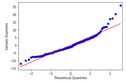
`fig4=sm.qqplot(reg3.resid, line='r')`

The qqplot shows that the residuals generally follow a straight line, but deviate at the lower and higher quantiles. This indicates that our residuals did not follow perfect normal distribution. This could mean that the curvilinear association that we observed in our scatter plot may not be fully estimated by the quadratic alcohol consumption rate term. There might be other explanatory variables that we might consider including in our model, that could improve estimation of the observed curvilinearity.

standardized residuals for all observations:

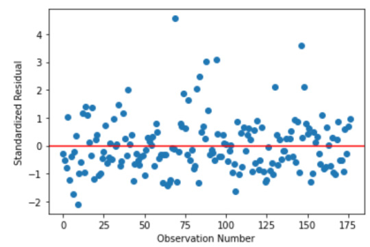
stdres=pd.DataFrame(reg3.resid_pearson) plt.plot(stdres, 'o', ls='None') l = plt.axhline(y=0, color='r') plt.ylabel('Standardized Residual') plt.xlabel('Observation Number')

Most of the residuals fall within one standard deviation of the mean, but there're also many residuals up to 2 standard diviations below the mean and there are several extreme outliers more than 3 standard diviations above the mean.

leverage plot:

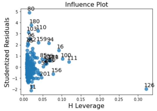
fig3=sm.graphics.influence_plot(reg3, size=8) print(fig3)

There are many observations with residuals greater than 2, which means that there are many outliers, but they have small or close to zero leverage values, meaning that although they are outlying observations, they do not have an undue influence on the estimation of the regression model. Only one observation has a high leverage and residual about -2, so we can't call it an outlier, which means that we don't have any observations that are both high leverage and outliers.

[research-regression]

data['alcconsumption'] = data['alcconsumption'].apply(lambda x: x - data['alcconsumption'].mean()) data['alcconsumption'].mean()

-1.0010010838241952e-15

[research-regression]

Basic Linear Regression Model Results

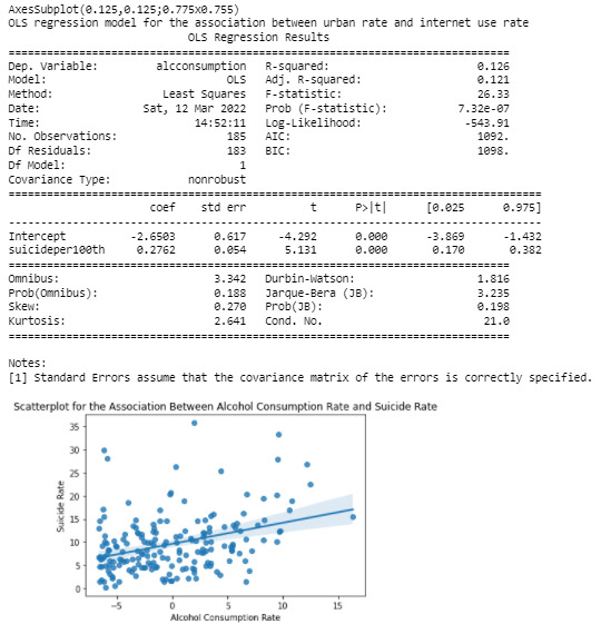
The results of the linear regression model indicated that suicide (Beta=0.28, p=.001) was significantly and positively associated with the rate of alcohol consumption. However, there is a heteroscedasticity.

[research-regression]

Basic Linear Regression Model

Hypothesis : Suicide rate is significantly associated with Alcohol Consumption Rate.

Response Variable: Suicide Rate, Explanatory Variable : Alcohol Consumption rate

Program

import pandas as pd import numpy as np import statsmodels.api import statsmodels.formula.api as smf import seaborn import matplotlib.pyplot as plt pd.set_option('display.float_format', lambda x:'%.2f'%x) data = pd.read_csv('gapminder.csv') data = data[["alcconsumption", "suicideper100th"]].dropna() data['alcconsumption'] = data['alcconsumption'].apply(lambda x: x - data['alcconsumption'].mean()) data['suicideper100th'] = pd.to_numeric(data['suicideper100th'], errors='coerce') data['alcconsumption'] = pd.to_numeric(data['alcconsumption'], errors='coerce') scat1 = seaborn.regplot(x="alcconsumption", y="suicideper100th", scatter=True, data=data) plt.xlabel('Alcohol Consumption Rate') plt.ylabel('Suicide Rate') plt.title ('Scatterplot for the Association Between Alcohol Consumption Rate and Suicide Rate') print(scat1) print ("OLS regression model for the association between urban rate and internet use rate") reg1 = smf.ols('alcconsumption ~ suicideper100th', data=data).fit() print (reg1.summary())

Output

[research-regression]

Measures

The level of misconception about issues around the world was measured by the percentage of wrong answers to the questionnaire compared to randomly choosing the option. The questionnaire consists of 18 fact-based questions regarding issues affecting people around the world today and presents the most commonly held misconceptions. Each question has three answers scaling as correct, incorrect and very wrong. So, only one answer can be regarded as the fact of the absence of misconception. To remove the probability of answering by chance the results were compared to randomly choosing the answer (1/3).

[research-regression]

Procedure

The data was collected by a questionnaire that consists of 18 important fact-based ABC-questions regarding issues affecting people around the world today. The surveys were conducted in October 2019 using Ipsos MORI survey platform.

[research-regression]

Sample

The sample is from Global Misconception Study 2019, a study that examines the knowledge of people in countries around the world regarding a broad range of important development topics using the Sustainable Development Goals as a common framework. Participants (N=15500) are from 31 countries: UAE, Argentina, Australia, Belgium, Brazil, Canada, China, Colombia, Germany, Egypt, Spain, France, Great Britain, Hungary, Indonesia, Italy, Jordan, Japan, South Korea, Morocco, Mexico, Malaysia, Peru, Poland, Romania, Russia, Saudi Arabia, Sweden, Singapore, Turkey, United States.