learner0010

[learner0010]

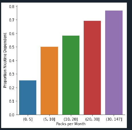
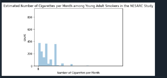
Number of Cigarettes per month vs count is the univariate graph and the proportion of Nicotine dependents vs Packs per month is the Bi Variate graph.

Univariate graph - It displays withonly one variable. Here it displays how the young adults smoke cigarttes per month. we can see that the Max cigarettes smoked is 400 per month and it can be as less as 10 for some months which indicate there is a huge standard deviation

Bi Variate graph - It displays Nicotine dependents vs Packs per month. we can see that Max packs of 147 per month is used by 75% people. Also less smokers use 5 packs which amount to 25% people. The trend we can see is that the high smokers are in the Maximum range of 75%.

Below is the programming code used.

import pandas import numpy import seaborn import matplotlib.pyplot as plt

any additional libraries would be imported here

Set PANDAS to show all columns in DataFrame

pandas.set_option('display.max_columns', None)

Set PANDAS to show all rows in DataFrame

pandas.set_option('display.max_rows', None)

bug fix for display formats to avoid run time errors

pandas.set_option('display.float_format', lambda x:'%f'%x)

data = pandas.read_csv('nesarc_pds.csv', low_memory=False)

print(len(data)) #number of observations (rows) print(len(data.columns)) # number of variables (columns)

checking the format of your variables

data['ETHRACE2A'].dtype

setting variables you will be working with to numeric (updated)

data['TAB12MDX'] = pandas.to_numeric(data['TAB12MDX']) data['CHECK321'] = pandas.to_numeric(data['CHECK321']) data['S3AQ3B1'] = pandas.to_numeric(data['S3AQ3B1']) data['S3AQ3C1'] = pandas.to_numeric(data['S3AQ3C1']) data['AGE'] = pandas.to_numeric(data['AGE'])

subset data to young adults age 18 to 25 who have smoked in the past 12 months

sub1=data[(data['AGE']>=18) & (data['AGE']<=25) & (data['CHECK321']==1)]

make a copy of my new subsetted data

sub2 = sub1.copy()

SETTING MISSING DATA

recode missing values to python missing (NaN)

sub2['S3AQ3B1']=sub2['S3AQ3B1'].replace(9, numpy.nan)

recode missing values to python missing (NaN)

sub2['S3AQ3C1']=sub2['S3AQ3C1'].replace(99, numpy.nan)

recode1 = {1: 6, 2: 5, 3: 4, 4: 3, 5: 2, 6: 1} sub2['USFREQ']= sub2['S3AQ3B1'].map(recode1)

recode2 = {1: 30, 2: 22, 3: 14, 4: 5, 5: 2.5, 6: 1} sub2['USFREQMO']= sub2['S3AQ3B1'].map(recode2)

A secondary variable multiplying the number of days smoked/month and the approx number of cig smoked/day

sub2['NUMCIGMO_EST']=sub2['USFREQMO'] * sub2['S3AQ3C1']

univariate bar graph for categorical variables

First hange format from numeric to categorical

sub2["TAB12MDX"] = sub2["TAB12MDX"].astype('category')

seaborn.countplot(x="TAB12MDX", data=sub2) plt.xlabel('Nicotine Dependence past 12 months') plt.title('Nicotine Dependence in the Past 12 Months Among Young Adult Smokers in the NESARC Study')

Univariate histogram for quantitative variable:

seaborn.distplot(sub2["NUMCIGMO_EST"].dropna(), kde=False); plt.xlabel('Number of Cigarettes per Month') plt.title('Estimated Number of Cigarettes per Month among Young Adult Smokers in the NESARC Study')

Code for Week 4 Python Lesson 3 - Measures of Center & Spread

standard deviation and other descriptive statistics for quantitative variables

print ('describe number of cigarettes smoked per month') desc1 = sub2['NUMCIGMO_EST'].describe() print (desc1)

c1= sub2.groupby('NUMCIGMO_EST').size() print (c1)

print ('describe nicotine dependence') desc2 = sub2['TAB12MDX'].describe() print (desc2)

c1= sub2.groupby('TAB12MDX').size() print (c1)

print ('mode') mode1 = sub2['TAB12MDX'].mode() print (mode1)

print ('mean') mean1 = sub2['NUMCIGMO_EST'].mean() print (mean1)

print ('std') std1 = sub2['NUMCIGMO_EST'].std() print (std1)

print ('min') min1 = sub2['NUMCIGMO_EST'].min() print (min1)

print ('max') max1 = sub2['NUMCIGMO_EST'].max() print (max1)

print ('median') median1 = sub2['NUMCIGMO_EST'].median() print (median1)

print ('mode') mode1 = sub2['NUMCIGMO_EST'].mode() print (mode1)

c1= sub2.groupby('TAB12MDX').size() print (c1)

p1 = sub2.groupby('TAB12MDX').size() * 100 / len(data) print (p1)

c2 = sub2.groupby('NUMCIGMO_EST').size() print (c2)

p2 = sub2.groupby('NUMCIGMO_EST').size() * 100 / len(data) print (p2)

A secondary variable multiplying the number of days smoked per month and the approx number of cig smoked per day

A secondary variable multiplying the number of days smoked per month and the approx number of cig smoked per day

sub2['PACKSPERMONTH']=sub2['NUMCIGMO_EST'] / 20

c2= sub2.groupby('PACKSPERMONTH').size() print (c2)

sub2['PACKCATEGORY'] = pandas.cut(sub2.PACKSPERMONTH, [0, 5, 10, 20, 30, 147])

change format from numeric to categorical

sub2['PACKCATEGORY'] = sub2['PACKCATEGORY'].astype('category')

print ('pack category counts') c7 = sub2['PACKCATEGORY'].value_counts(sort=False, dropna=True) print(c7)

print ('describe PACKCATEGORY') desc3 = sub2['PACKCATEGORY'].describe() print (desc3)

sub2['TAB12MDX'] = pandas.to_numeric(sub2['TAB12MDX'])

bivariate bar graph C->Q

seaborn.catplot(x="PACKCATEGORY", y="TAB12MDX", data=sub2, kind="bar", ci=None) plt.xlabel('Packs per Month') plt.ylabel('Proportion Nicotine Dependent')

creating 3 level smokegroup variable

def SMOKEGRP (row): if row['TAB12MDX'] == 1 : return 1 elif row['USFREQMO'] == 30 : return 2 else : return 3

sub2['SMOKEGRP'] = sub2.apply (lambda row: SMOKEGRP (row),axis=1)

c3= sub2.groupby('SMOKEGRP').size() print (c3)

creating daily smoking variable

def DAILY (row): if row['USFREQMO'] == 30 : return 1 elif row['USFREQMO'] != 30 : return 0

sub2['DAILY'] = sub2.apply (lambda row: DAILY (row),axis=1)

c4= sub2.groupby('DAILY').size() print (c4)

seaborn.catplot(x='ETHRACE2A', y='DAILY', data=sub2, kind="bar", ci=None) plt.xlabel('Ethnic Group') plt.ylabel('Proportion Daily Smokers')

you can rename categorical variable values for graphing if original values are not informative

first change the variable format to categorical if you haven’t already done so

sub2['ETHRACE2A'] = sub2['ETHRACE2A'].astype('category')

second create a new variable (PACKCAT) that has the new variable value labels

sub2['ETHRACE2A']=sub2['ETHRACE2A'].cat.rename_categories(["White", "Black", "NatAm", "Asian", "Hispanic"])

bivariate bar graph C->C

seaborn.catplot(x='ETHRACE2A', y='DAILY', data=sub2, kind="bar", ci=None) plt.xlabel('Ethnic Group') plt.ylabel('Proportion Daily Smokers')

check to see if missing data were set to NaN

print ('counts for S3AQ3C1 with 99 set to NAN and number of missing requested') c4 = sub2['S3AQ3C1'].value_counts(sort=False, dropna=False) print(c4)

print ('counts for TAB12MDX - past 12 month nicotine dependence') c5 = sub2['TAB12MDX'].value_counts(sort=False) print(c5)

[learner0010]

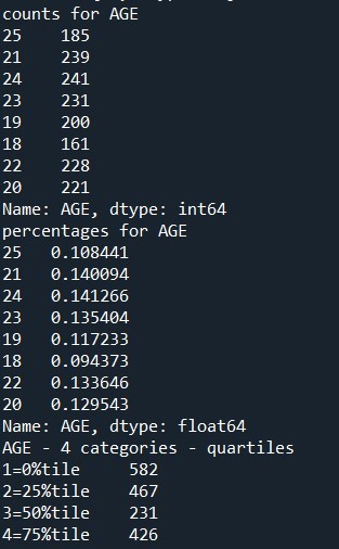
This is a description of the percentage of smoking in youg adults. below is the python code.

import pandas import numpy

any additional libraries would be imported here

data = pandas.read_csv('nesarc_pds.csv', low_memory=False)

bug fix for display formats to avoid run time errors

pandas.set_option('display.float_format', lambda x:'%f'%x)

setting variables you will be working with to numeric (updated)

data['TAB12MDX'] = pandas.to_numeric(data['TAB12MDX']) data['CHECK321'] = pandas.to_numeric(data['CHECK321']) data['S3AQ3B1'] = pandas.to_numeric(data['S3AQ3B1']) data['S3AQ3C1'] = pandas.to_numeric(data['S3AQ3C1']) data['AGE'] = pandas.to_numeric(data['AGE'])

subset data to young adults age 18 to 25 who have smoked in the past 12 months

sub1=data[(data['AGE']>=18) & (data['AGE']<=25) & (data['CHECK321']==1)]

make a copy of my new subsetted data

sub2 = sub1.copy()

print ('counts for original S3AQ3B1') c1 = sub2['S3AQ3B1'].value_counts(sort=False, dropna=False) print(c1)

recode missing values to python missing (NaN)

sub2['S3AQ3B1']=sub2['S3AQ3B1'].replace(9, numpy.nan) sub2['S3AQ3C1']=sub2['S3AQ3C1'].replace(99, numpy.nan)

if you want to include a count of missing add ,dropna=False after sort=False

print ('counts for S3AQ3B1 with 9 set to NAN and number of missing requested') c2 = sub2['S3AQ3B1'].value_counts(sort=False, dropna=False) print(c2)

coding in valid data

recode missing values to numeric value, in this example replace NaN with 11

sub2['S2AQ8A'].fillna(11, inplace=True)

recode 99 values as missing

sub2['S2AQ8A']=sub2['S2AQ8A'].replace(99, numpy.nan)

print ('S2AQ8A with Blanks recoded as 11 and 99 set to NAN')

check coding

chk2 = sub2['S2AQ8A'].value_counts(sort=False, dropna=False) print(chk2) ds2= sub2["S2AQ8A"].describe() print(ds2)

recoding values for S3AQ3B1 into a new variable, USFREQ

recode1 = {1: 6, 2: 5, 3: 4, 4: 3, 5: 2, 6: 1} sub2['USFREQ']= sub2['S3AQ3B1'].map(recode1)

recoding values for S3AQ3B1 into a new variable, USFREQMO

recode2 = {1: 30, 2: 22, 3: 14, 4: 5, 5: 2.5, 6: 1} sub2['USFREQMO']= sub2['S3AQ3B1'].map(recode2)

secondary variable multiplying the number of days smoked/month and the approx number of cig smoked/day

sub2['NUMCIGMO_EST']=sub2['USFREQMO'] * sub2['S3AQ3C1']

examining frequency distributions for age

print('counts for AGE') c5 = sub2['AGE'].value_counts(sort=False) print(c5) print('percentages for AGE') p5 = sub2['AGE'].value_counts(sort=False, normalize=True) print (p5)

quartile split (use qcut function & ask for 4 groups - gives you quartile split)

print ('AGE - 4 categories - quartiles') sub2['AGEGROUP4']=pandas.qcut(sub2.AGE, 4, labels=["1=0%tile","2=25%tile","3=50%tile","4=75%tile"]) c4 = sub2['AGEGROUP4'].value_counts(sort=False, dropna=True) print(c4)

categorize quantitative variable based on customized splits using cut function

sub2['AGEGROUP3'] = pandas.cut(sub2.AGE, [17, 20, 22, 25]) c5 = sub2['AGEGROUP3'].value_counts(sort=False, dropna=True) print(c5)

crosstabs evaluating which ages were put into which AGEGROUP3

print (pandas.crosstab(sub2['AGEGROUP3'], sub2['AGE']))

Summary - It is evident that there is a normal distribution of smokers where the smoker percentage increases at the age group of 19-24 and gradually decreases. Also it is intersting to note that the quarter percentage reduces for 3 quarters from pealk and then slightly increases. Here for the non available or missing data, we have ignored the missing data after converting it to NaN

[learner0010]

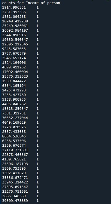
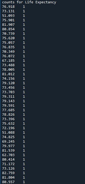
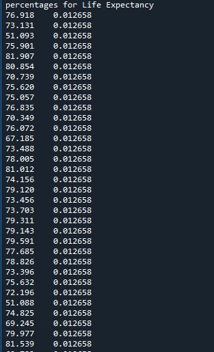
Program for understanding coreleation of income per person > $1300 & life expectancy > 50 years & employ rate > 50

import pandas

#import numpy

import os

# any additional libraries would be imported here

pwd= os.getcwd()

data = pandas.read_csv('gap minder.csv', low_memory=False)

#pandas.options.display.max_rows = None

#print (len(data)) #number of observations (rows)

#print (len(data.columns)) # number of variables (columns)

# checking the format of your variables

#print(data['incomeperperson'].dtype)

#setting variables you will be working with to numeric

data['incomeperperson'] = pandas.to_numeric(data['incomeperperson'],errors='coerce')

data['lifeexpectancy'] = pandas.to_numeric(data['lifeexpectancy'],errors='coerce')

data['armedforcesrate'] = pandas.to_numeric(data['armedforcesrate'],errors='coerce')

data['employrate'] = pandas.to_numeric(data['employrate'],errors='coerce')

data['internetuserate'] = pandas.to_numeric(data['internetuserate'],errors='coerce')

#print ('counts for Income of Person')

#counts and percentages (i.e. frequency distributions) for each variable

c1 = data['incomeperperson'].value_counts(sort=False)

#print (c1)

#print ('percentages for Income of Person')

p1 = data['incomeperperson'].value_counts(sort=False, normalize=True)

#print (p1)

#print ('counts for Life Expectancy')

c2 = data['lifeexpectancy'].value_counts(sort=False)

#print(c2)

#print ('percentages for Life Expectancy')

p2 = data['lifeexpectancy'].value_counts(sort=False, normalize=True)

#print (p2)

#print ('counts for Armed Force rate')

c3 = data['armedforcesrate'].value_counts(sort=False)

#print(c3)

#print ('percentages for Armed forces rate')

p3 = data['armedforcesrate'].value_counts(sort=False, normalize=True)

#print (p3)

#print ('counts for Employee rate')

c4 = data['employrate'].value_counts(sort=False)

#print(c4)

#print ('percentages for Employee Rate')

p4 = data['employrate'].value_counts(sort=False, normalize=True)

#print (p4)

#subset data to income per person >1300 and Life expectancy >50 and Employee rate >50

sub1=data[(data['incomeperperson']>1300) & (data['lifeexpectancy']>50) & (data['employrate']>50)]

sub2 = sub1.copy()

# frequency distributions on new sub2 data frame

c5 = sub2['incomeperperson'].value_counts(sort=False)

print ('counts for Income of person')

print (c5)

print ('percentages for Income of Person')

p5 = sub2['incomeperperson'].value_counts(sort=False, normalize=True)

print (p5)

print ('counts for Life Expectancy')

c6 = sub2['lifeexpectancy'].value_counts(sort=False)

print(c6)

print ('percentages for Life Expectancy')

p6 = sub2['lifeexpectancy'].value_counts(sort=False, normalize=True)

print (p6)

print ('counts for Armed Force rate')

c7 = sub2['armedforcesrate'].value_counts(sort=False)

print(c7)

print ('percentages for Armed forces rate')

p7 = sub2['armedforcesrate'].value_counts(sort=False, normalize=True)

print (p7)

print ('counts for Employee rate')

c8 = sub2['employrate'].value_counts(sort=False)

print(c8)

print ('percentages for Employee Rate')

p8 = sub2['employrate'].value_counts(sort=False, normalize=True)

print (p8)

output display

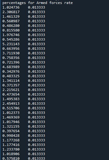
Summary – The Frequency distribution was made on variables income per person, life expectancy & employ rate .

The number of persons above income of 1300 USD monthly and having a life expectancy of above 50 is very less at 1.2%. Also we find that the employment rate is also less at 1.2-2.5%. Also we see that the values taken is at constant level of 1 or 2 %. The missing data is not considered further for analysis and the corelation is made on the available data. This means that for people with very less means to have a good standard life have very less life expectancy.

[learner0010]

Life expectancy - Relation with Armed forces and Employment rate

STEP 1: Choose a data set that you would like to work with.

 

Dataset I chose to work with is Gapminder .

STEP 2. Identify a specific topic of interest

I find interest in the corelation between armed forces rate and life expectancy.

STEP 3. Prepare a codebook of your own

Variable Name Description of Indicator Main Source

incomeperperson 2010 Gross Domestic Product per capita in constant 2000 US$. The

inflation but not the differences in the cost of living between countries

has been taken into account.

World Bank Work Development

Indicators

alcconsumption 2008 alcohol consumption per adult (age 15+), litres

Recorded and estimated average alcohol consumption, adult (15+) per

capita consumption in litres pure alcohol

WHO

armedforcesrate Armed forces personnel (% of total labor force) Work Development Indicators

breastcancerper100TH 2002 breast cancer new cases per 100,000 female

Number of new cases of breast cancer in 100,000 female residents

during the certain year.

ARC (International Agency for

Research on Cancer)

co2emissions 2006 cumulative CO2 emission (metric tons), Total amount of CO2

emission in metric tons since 1751.

CDIAC (Carbon Dioxide

Information Analysis Center)

femaleemployrate 2007 female employees age 15+ (% of population)

Percentage of female population, age above 15, that has been

employed during the given year.

International Labour

Organization

employrate 2007 total employees age 15+ (% of population)

Percentage of total population, age above 15, that has been employed

during the given year.

International Labour

Organization

HIVrate 2009 estimated HIV Prevalence % - (Ages 15-49)

Estimated number of people living with HIV per 100 population of age

group 15-49.

UNAIDS online database

Internetuserate 2010 Internet users (per 100 people)

Internet users are people with access to the worldwide network.

World Bank

lifeexpectancy 2011 life expectancy at birth (years)

The average number of years a newborn child would live if current

mortality patterns were to stay the same.

1. Human Mortality Database,

2. World Population Prospects:

3. Publications and files by

history prof. James C Riley

4. Human Lifetable Database

STEP 4. Identify a second topic that you would like to explore in terms of its association with your original topic.

I also find interesting to corelate Employrate with respect to life expectancy

 

STEP 5. Add questions/items/variables documenting this second topic to your personal codebook.

 

Added in the first snapshot (combined)

STEP 6. Perform a literature review to see what research has been previously done on this topic. Use sites such as Google Scholar (http://scholar.google.com) to search for published academic work in the area(s) of interest. Try to find multiple sources, and take note of basic bibliographic information

Employment rate - OECD Data

https://data.oecd.org › emp › employment-rate

 

Life Expectancy - Our World in Data

https://ourworldindata.org › life-expectancy

 

Life expectancy - Wikipedia

https://en.wikipedia.org › wiki › Life_expectancy

 

FastStats - Life Expectancy - CDC

 

 

Step 7 : Based on your literature review, develop a hypothesis about what you believe the association might be between these topics. Be sure to integrate the specific variables you selected into the hypothesis.

 

Based on the literature review, it is interesting to note that life expectancy increases as the armed force rate increases. This is because the govt is stable in the countries and citizens live well there. Also the employment rate tends to increase there as the life style improves and more stability and prosperity is brought in by goverments.