jcvallier

[jcvallier]

Data Analysis Capstone - Week 3

This week I am discussing my analysis of Tanzania water wells. Analysis

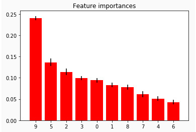
After using the random forest algorithm, the following 10 variables were ranked for importance using the scikit-learn feature importance function (use the feature table to reference each variable name and description), see chart below. The top four variables were: (9) gps_height, (5) quantity, (2) lga, (3) construction_year.  

Gps_height variable :

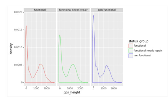
The following is a density plot of of gps_height.  The target variables of functional, functional needs repair, and nonfunctional all have similar plots, with a spike at zero and another near 1500 meters(units assumed).  

This indicates that gps_height alone is not sufficient to determine between the target variables.Given that gps_height is the most important feature, there is probably a strong relationship with other variables in the dataset.  

Quantity variable :

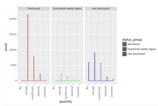
For the quantity variable there is more non functional dry wells than functional dry or functional needs repair dry.  It is also of note that non functional enough is the largest count for functional, functional needs repair, and non functional.  It is important to note, it is twice more likely to be functional when the quantity is functional enough versus non-functional enough.

Lga variable:

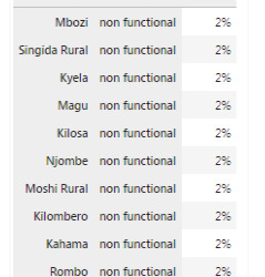
Lga Is a geographical territory. No one region had more non functionals in the top ten, see table below.   

Construction_Year variable -

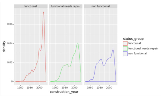
The range of dates included 1960 through 2013 (excluding nulls 20,710).  This variable revels that the vast majority of wells were set up in the last decade.  It is interesting to see that there are more significant spikes in functional needs repair and non functional repair around 1980.  

[jcvallier]

Data Analysis -  Capstone Week 2

Methods

Sample:

Data was collected  from 2002 to 2013 by Taarifa and the Tanzanian Ministry of Water on water pumps in through out Tanzanian.  The data collected was designed to understand which waterpoints will fail and where they can improve maintenance operations and ensure that clean, potable water is available to local communities. The wells are classified into three categories: functional, functional needs repair, and not functional.  

Variables:

The following variables were selected to train and test the model.

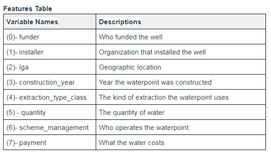
The following are the target variables, were ‘not functional’ is the key target to be predicted for feature importance.

Statistical Analyses:

Training & Test Split with cross validation

After the key variables were selected above, the remaining dataset was split into a training set and a test set.  The dataset training to test split was 75% and 25%, respectively.

A 10 k-fold cross validation was done with on 8 features with the sequential feature selection greedy algorithm.  This was done to observe which features contributed to the overall accuracy score.

Random Forest Algorithm Explained:

Random Forest is an ensemble approach with decision trees.  The ensemble method takes a group of weak learners and together form a strong learner.

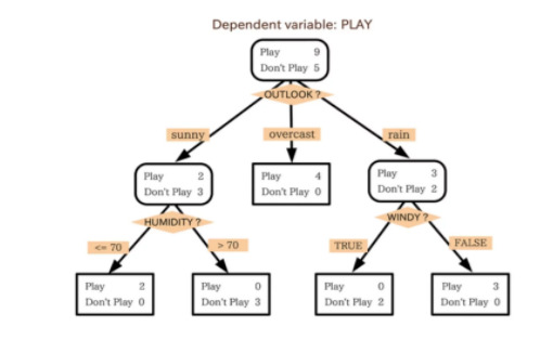
Therefore, a decision tree which, in ensemble terms, corresponds to our weak learner, and takes your target data entered at the top and then gets traverses down the tree where it is bucketed into smaller and smaller sets until your target cannot be split any further.

In the example below, the tree advises us, based upon weather conditions, whether to play ball. For example, if the outlook is sunny and the humidity is less than or equal to 70, then it’s probably OK to play. See diagram below..

As shown in diagram below, random forest is a collection of the decision trees where the data are randomly shuffled into subsets and decision trees are formed for each random split.   

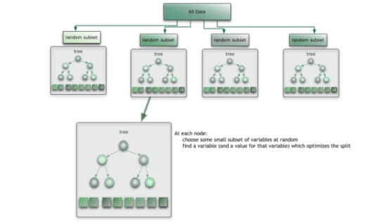
Once the trees have been split, a majority vote of the mode is used for categorical predictor and mean for quantitative.  The result is a predictive model, that due to the ensemble method, creates a stronger predictive model that avoids overfitting the data due to its randomness.

See the example below, where each decision tree is shown as a gray curve. Each gray curve (a weak learner) is a fair approximation to the underlying data. The red curve (the ensemble “strong learner”) can be seen to be a much better approximation to the underlying data.

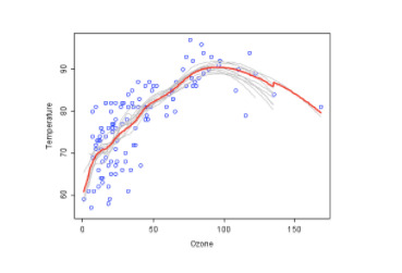
Random forests can be used to rank the importance of variables in a regression or classification problem in a natural way, where features which produce large values for this score are ranked as more important than features which produce small values.

This method of determining variable importance has some drawbacks. For data including categorical variables with different number of levels, random forests are biased in favor of those attributes with more levels. Using additional unbiased trees or training on a balanced data set can help with this problem.

How Random Forest is being applied to the dataset :

When setting the parameters of random forest, 125 trees were selected for a robust generalized score.  Additionally, class weight was selected as ‘balanced’ as the key target of ‘not functional’ was under-represented in the training set and additional weight for predication would be given to the other categories of ‘functional’, and ‘functional needs repair’ if left unadjusted.

Source: http://blog.citizennet.com/blog/2012/11/10/random-forests-ensembles-and-performance-metric

[jcvallier]

Data Analysis - Capstone Week 1

In the preparation of writing a data analysis paper for this capstone.  This week we are asked to provide a (1) project title, (2) a research question with my motivation for answering the question, and (3)  potential implications of answering the research question.

(1) Project Title:  Identifying the best predictors which may cause water pumps to fail in Tanzania using a random forest machine learning algorithm.

(2) Research Question:  Can a random forest machine learning algorithm predicts which water pumps will fail in Tanzania, to improve improve maintenance operations that provide clean, potable water for local communities?  I plan on using the this method to best identify possible factors.

(3) Implications for research question: By answering this question, this could lead to an improved maintenance schedule that could decrease the amount of water pump failures, and lead to more potable clean water for local communities.

[jcvallier]

Machine Learning for Data Analysis - Week 4

This week we focused on K-means unsupervised learning algorithm.  K-means clustering aims to partition n observations into k - clusters in which each observation belongs to the cluster with the nearest mean, serving as a prototype of the cluster.  These clusters are not labeled and need the user to examine closely the related variables to understand the characteristics.  

I did this assignment on red wine quality dataset found in UCI machine learning data set repository. 

I didn’t have any N/A values to manage:

angeIndex: 1599 entries, 0 to 1598 Data columns (total 12 columns): fixed acidity           1599 non-null float64 volatile acidity        1599 non-null float64 citric acid             1599 non-null float64 residual sugar          1599 non-null float64 chlorides               1599 non-null float64 free sulfur dioxide     1599 non-null float64 total sulfur dioxide    1599 non-null float64 density                 1599 non-null float64 pH                      1599 non-null float64 sulphates               1599 non-null float64 alcohol                 1599 non-null float64 quality                 1599 non-null int64 dtypes: float64(11), int64(1)

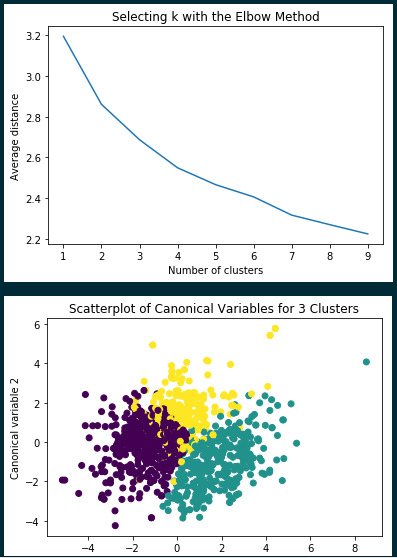
Looking at the elbow method for electing how many k clusters, it looks like between 2 and 4 looks optional.  I ran a Turkey HSD test for 3 and 4 clusters. with the best results for 3 clusters.

Clustering variable means by cluster              index  fixed acidity  volatile acidity  citric acid  \ cluster                                                             0        852.964981      -0.613198          0.523980    -0.766575   1        735.110787       0.972455         -0.724979     1.044456   2        710.416031      -0.000537          0.037230     0.174129  

        residual sugar  chlorides  free sulfur dioxide  total sulfur dioxide  \ cluster                                                                         0             -0.213666  -0.157534            -0.246837             -0.351623   1              0.006391   0.270782            -0.473441             -0.497666   2              0.489412   0.020018             1.046380              1.276995  

         density        pH  sulphates   alcohol   quality   cluster                                                     0       -0.384480  0.590419  -0.315140 -0.005503 -0.187766   1        0.368134 -0.734856   0.576452  0.413372  0.570021   2        0.385615 -0.199118  -0.121968 -0.521363 -0.447425  

Here cluster 1 has the best quality with the highest alcohol, sulphates, and fixed acidity.  Cluster 0 is close to the mean quality and has the second highest alcohol (near average), however other qualities vary.  Cluster 2 has the lowest quality and the lowest alcohol, but also vary in other qualities.

Running a post hoc test again we can see the clusters rejected the null hypthesis and the means and standard deviations vary. 

means for alcohol by cluster         alcohol_y cluster           0        -0.060487 1         0.422731 2        -0.513167 standard deviations for alcohol by cluster         alcohol_y cluster           0         0.949251 1         1.045772 2         0.728444 Multiple Comparison of Means - Tukey HSD,FWER=0.05 ============================================= group1 group2 meandiff  lower   upper  reject ---------------------------------------------  0      1     0.4832   0.3003  0.6661  True  0      2    -0.4527  -0.6481 -0.2573  True  1      2    -0.9359  -1.1472 -0.7246  True

In summary, it looks like I was able to determine three categories of wine: high quality, middle quality, and low quality using K-means analysis.  This allowed me to understand the characteristics of each category and to perhaps predict whether a bottle of wine will be high quality.  Here is my code:

@author: jcvall """

from pandas import Series, DataFrame import pandas as pd import numpy as np import matplotlib.pylab as plt from sklearn.model_selection import train_test_split from sklearn import preprocessing from sklearn.cluster import KMeans

#%% """ Data Management """ #%cd /Users/jcvall/Google Drive/Education/Python & Data Science/Mac - Python data = pd.read_csv("winequality-red.csv",sep=";")

# subset clustering variables data.info()

# preprocess dataframe

clustervar = data

# standardize clustering variables to have mean=0 and sd=1

clustervar['fixed acidity']=preprocessing.scale(clustervar['fixed acidity'].astype('float64')) clustervar['volatile acidity']=preprocessing.scale(clustervar['volatile acidity'].astype('float64')) clustervar['citric acid']=preprocessing.scale(clustervar['citric acid'].astype('float64')) clustervar['residual sugar']=preprocessing.scale(clustervar['residual sugar'].astype('float64')) clustervar['chlorides']=preprocessing.scale(clustervar['chlorides'].astype('float64')) clustervar['free sulfur dioxide']=preprocessing.scale(clustervar['free sulfur dioxide'].astype('float64')) clustervar['total sulfur dioxide']=preprocessing.scale(clustervar['total sulfur dioxide'].astype('float64')) clustervar['density']=preprocessing.scale(clustervar['density'].astype('float64')) clustervar['pH']=preprocessing.scale(clustervar['pH'].astype('float64')) clustervar['sulphates']=preprocessing.scale(clustervar['sulphates'].astype('float64')) clustervar['alcohol']=preprocessing.scale(clustervar['alcohol'].astype('float64')) clustervar['quality']=preprocessing.scale(clustervar['quality'].astype('float64'))                                                                                                                

# split data into train and test sets clus_train, clus_test = train_test_split(clustervar, test_size=.3, random_state=111)

# k-means cluster analysis for 1-9 clusters                                                           from scipy.spatial.distance import cdist clusters=range(1,10) meandist=[]

for k in clusters:    model=KMeans(n_clusters=k)    model.fit(clus_train)    clusassign=model.predict(clus_train)    meandist.append(sum(np.min(cdist(clus_train, model.cluster_centers_, 'euclidean'), axis=1))    / clus_train.shape[0])

#%%

""" Plot average distance from observations from the cluster centroid to use the Elbow Method to identify number of clusters to choose """

plt.plot(clusters, meandist) plt.xlabel('Number of clusters') plt.ylabel('Average distance') plt.title('Selecting k with the Elbow Method') plt.show()

# Interpret 3 cluster solution model3=KMeans(n_clusters=5) model3.fit(clus_train) clusassign=model3.predict(clus_train) # plot clusters

from sklearn.decomposition import PCA pca_2 = PCA(2) plot_columns = pca_2.fit_transform(clus_train) plt.scatter(x=plot_columns[:,0], y=plot_columns[:,1], c=model3.labels_,) plt.xlabel('Canonical variable 1') plt.ylabel('Canonical variable 2') plt.title('Scatterplot of Canonical Variables for 3 Clusters') plt.show()

#%% """ BEGIN multiple steps to merge cluster assignment with clustering variables to examine cluster variable means by cluster """ # create a unique identifier variable from the index for the # cluster training data to merge with the cluster assignment variable clus_train.reset_index(level=0, inplace=True) # create a list that has the new index variable cluslist=list(clus_train['index']) # create a list of cluster assignments labels=list(model3.labels_) # combine index variable list with cluster assignment list into a dictionary newlist=dict(zip(cluslist, labels)) newlist # convert newlist dictionary to a dataframe newclus=DataFrame.from_dict(newlist, orient='index') newclus # rename the cluster assignment column newclus.columns = ['cluster']

# now do the same for the cluster assignment variable # create a unique identifier variable from the index for the # cluster assignment dataframe # to merge with cluster training data newclus.reset_index(level=0, inplace=True) # merge the cluster assignment dataframe with the cluster training variable dataframe # by the index variable merged_train=pd.merge(clus_train, newclus, on='index') merged_train.head(n=100) # cluster frequencies merged_train.cluster.value_counts()

#%%

""" END multiple steps to merge cluster assignment with clustering variables to examine cluster variable means by cluster """

# FINALLY calculate clustering variable means by cluster clustergrp = merged_train.groupby('cluster').mean() print ("Clustering variable means by cluster") print(clustergrp)

#%%

# validate clusters in training data by examining cluster differences in alcohol using ANOVA # first have to merge alcohol with clustering variables and cluster assignment data alcohol_data=data['alcohol'] # split alcohol data into train and test sets alcohol_train, alcohol_test = train_test_split(alcohol_data, test_size=.3, random_state=123) alcohol_train1=pd.DataFrame(alcohol_train) alcohol_train1.reset_index(level=0, inplace=True) merged_train_all=pd.merge(alcohol_train1, merged_train, on='index') sub1 = merged_train_all[['alcohol_y', 'cluster']]

import statsmodels.formula.api as smf import statsmodels.stats.multicomp as multi

alcoholmod = smf.ols(formula='alcohol_y ~ C(cluster)', data=sub1).fit() print (alcoholmod.summary())

print ('means for alcohol by cluster') m1= sub1.groupby('cluster').mean() print (m1)

print ('standard deviations for alcohol by cluster') m2= sub1.groupby('cluster').std() print (m2)

mc1 = multi.MultiComparison(sub1['alcohol_y'], sub1['cluster']) res1 = mc1.tukeyhsd() print(res1.summary())

[jcvallier]

Machine Learning for Data Analysis - Week 3

This week we studied lasso regression. A regression algorithm that selects the best variable for better predictability.  Lasso Regression is able to achieve this goal by forcing the sum of the absolute value of the regression coefficients to be less than a fixed value, which forces certain coefficients to be set to zero, effectively choosing a simpler model that does not include those coefficients. 

I used the red wine data set where I am predicting the highest quality of wine, based on wine characteristics.

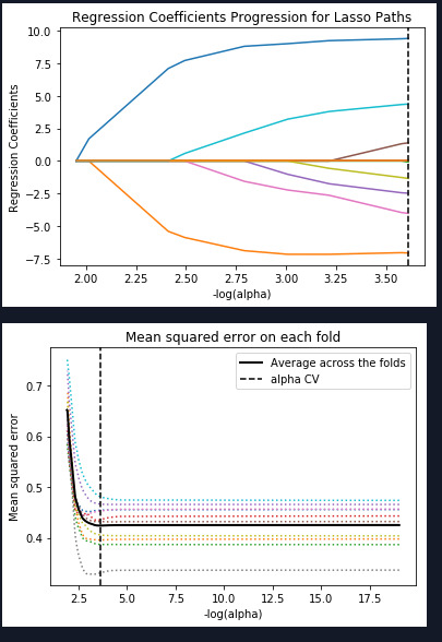
As you can see above the mean squared error is close to each fold with the exception of one that is very low MSE.  The training and test MSE are within .02 and the R square test is also within .02 of the training.  The lasso regression model has an R square of .34 in the test which means these variables can explain approximately 34% of the variable qualities of wine.

training data MSE 0.41434260704 test data MSE 0.432483541099 training data R-square 0.362115137182 test data R-square 0.340279344086

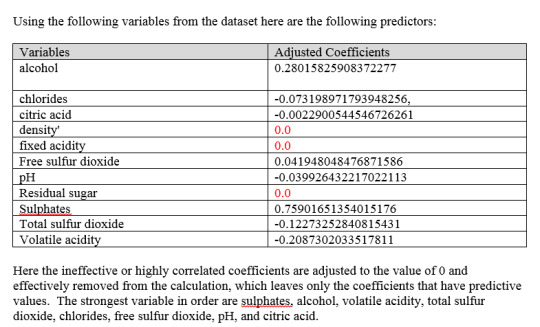
In summary the model shows us that the there is a relationship with Sulphates and Alcohol and red wine quality with other factors playing a lesser role.

Code:

#from pandas import Series, DataFrame import pandas as pd import numpy as np import matplotlib.pylab as plt from sklearn.cross_validation import train_test_split from sklearn.linear_model import LassoLarsCV import os

#Load the dataset os.chdir('C:/Users/10040207/myproject/Upload') data = pd.read_csv("winequality-red.csv",sep=';')

#%%

#select predictor variables and target variable as separate data sets   target = data['quality'] data.drop('quality',axis=1,inplace=True) predvar= data #%% # standardize predictors to have mean=0 and sd=1 predictors=predvar from sklearn import preprocessing predictors['fixeed acidity']=preprocessing.scale(predictors['fixed acidity'].astype('float64')) predictors['volatile acidity']=preprocessing.scale(predictors['volatile acidity'].astype('float64')) predictors['citric acid']=preprocessing.scale(predictors['citric acid'].astype('float64')) predictors['residual sugar']=preprocessing.scale(predictors['residual sugar'].astype('float64')) predictors['chlorides']=preprocessing.scale(predictors['chlorides'].astype('float64')) predictors['free sulfur dioxide']=preprocessing.scale(predictors['free sulfur dioxide'].astype('float64')) predictors['total sulfur dioxide']=preprocessing.scale(predictors['total sulfur dioxide'].astype('float64')) predictors['density']=preprocessing.scale(predictors['density'].astype('float64')) predictors['pH']=preprocessing.scale(predictors['pH'].astype('float64')) predictors['alcohol']=preprocessing.scale(predictors['alcohol'].astype('float64'))

#%% # split data into train and test sets pred_train, pred_test, tar_train, tar_test = train_test_split(predictors, target,                                                              test_size=.3, random_state=111)

# specify the lasso regression model model=LassoLarsCV(cv=10, precompute=False).fit(pred_train,tar_train) #%% # print variable names and regression coefficients dict(zip(predictors.columns, model.coef_))

#%% # plot coefficient progression m_log_alphas = -np.log10(model.alphas_) ax = plt.gca() plt.plot(m_log_alphas, model.coef_path_.T) plt.axvline(-np.log10(model.alpha_), linestyle='--', color='k',            label='alpha CV') plt.ylabel('Regression Coefficients') plt.xlabel('-log(alpha)') plt.title('Regression Coefficients Progression for Lasso Paths') #%% # plot mean square error for each fold m_log_alphascv = -np.log10(model.cv_alphas_) plt.figure() plt.plot(m_log_alphascv, model.cv_mse_path_, ':') plt.plot(m_log_alphascv, model.cv_mse_path_.mean(axis=-1), 'k',         label='Average across the folds', linewidth=2) plt.axvline(-np.log10(model.alpha_), linestyle='--', color='k',            label='alpha CV') plt.legend() plt.xlabel('-log(alpha)') plt.ylabel('Mean squared error') plt.title('Mean squared error on each fold')    #%%    

# MSE from training and test data from sklearn.metrics import mean_squared_error train_error = mean_squared_error(tar_train, model.predict(pred_train)) test_error = mean_squared_error(tar_test, model.predict(pred_test)) print ('training data MSE') print(train_error) print ('test data MSE') print(test_error)

# R-square from training and test data rsquared_train=model.score(pred_train,tar_train) rsquared_test=model.score(pred_test,tar_test) print ('training data R-square') print(rsquared_train) print ('test data R-square') print(rsquared_test)

[jcvallier]

Machine Learning for Data Analysis - Week 2

I continued with the red wine dataset this week to see if random forest can do a better job than decision trees.  I was able to get a marginal improvement from 0.978 for decision trees to 0.987 for random forest.  I used the quality variable as the target variable, where 1 is the highest rating and 0 is all other ratings.  The goal was to develop a random forest  model that can pick the best quality wine. Random Forest features ranking are as follows (higher the number the better). 

Features Rankfixed acidity0.065315 (9)volatile acidity0.109250 (3)citric acid0.104638 (4)residual sugar

0.0977009( 5)

chlorides0.059328 (10)free sulfur dioxide0.053690 (11)total sulfur dioxide0.072195 (7)density0.067850 (8)ph

0.093891 (6)

sulphates0.113916 (2)alcohol

0.162228 (1)

Summary -

The most important five features are Alcohol, sulphates, volatile acidity, Citric acid, and residual sugar.  The confusion matrix is as follows:

Confusion Matrix::

 [[632   0] [  7   1]]

The model correctly identified 632 that were correct classified as 0, 1 correctly classified  as 1.  Seven classified incorrectly when they indicate 0 but should have been 1.  Overall the model may need more examples but seems to do a good job.

Here is the code:

 from pandas import Series, DataFrame import pandas as pd import numpy as np import os import matplotlib.pylab as plt from sklearn.model_selection import train_test_split from sklearn.tree import DecisionTreeClassifier from sklearn.metrics import classification_report import sklearn.metrics  # Feature Importance from sklearn import datasets from sklearn.ensemble import ExtraTreesClassifier %matplotlib inline

 print(wine.dtypes) print(wine.describe())

#Split into training and testing sets

X_train,X_test,y_train,y_test = train_test_split(X,y,test_size=0.4,random_state=111)

col = X.columns

# fit an Extra Trees model to the data model = ExtraTreesClassifier() model.fit(X_train,y_train) # display the relative importance of each attribute features = model.feature_importances_ print(features)

pd.DataFrame(features,index=col,columns=['Features Rank'])

""" Running a different number of trees and see the effect  of that on the accuracy of the prediction """

trees=range(25) accuracy=np.zeros(25)

for idx in range(len(trees)):    classifier=RandomForestClassifier(n_estimators=idx + 1)    classifier=classifier.fit(X_train,y_train)    predictions=classifier.predict(X_test)    accuracy[idx]=sklearn.metrics.accuracy_score(y_test, predictions)    plt.cla() plt.plot(trees, accuracy)

[jcvallier]

Machine Learning for Data Analysis

I went to the UCI website to get an additional data set for the assignment. I choose red wine quality data.   A created a new variable for the where there is a 1 if it is the highest quality (8) or 0 if it is below 8.  

My variables are as such:

fixed acidity           X1 volatile acidity        X2 citric acid             X3 residual sugar          X3 chlorides               X4 free sulfur dioxide     X5 total sulfur dioxide    X6 density                 X7 pH                      x8 sulphates               X9 alcohol                 X10 quality                 X11 Highest_Q           X12

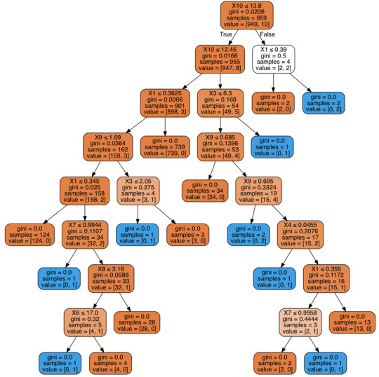
Decision Tree: 

My Code:

import pandas as pd import matplotlib.pyplot as plt import numpy as np import os from sklearn.model_selection import train_test_split from sklearn.tree import DecisionTreeClassifier from sklearn.metrics import classification_report import sklearn.metrics

wine = pd.read_csv('winequality-red.csv',sep=";")

wine['Highest_Q'] = wine['quality'].apply(lambda x: 0 if x < 8 else 1)

wine['quality'] = wine['quality'].astype('float64') wine['Highest_Q'] = wine['Highest_Q'].astype('float64') y = wine['Highest_Q'] wine.drop('quality',axis=1,inplace=True) wine.drop('Highest_Q',axis=1,inplace=True) X = wine

X_train,X_test,y_train,y_test = train_test_split(X,y,test_size=0.4,random_state=111)

classifier = DecisionTreeClassifier() classifier = classifier.fit(X_train,y_train)

predictions = classifier.predict(X_test)

sklearn.metrics.confusion_matrix(y_test,predictions)

sklearn.metrics.accuracy_score(y_test,predictions)

from sklearn.externals.six import StringIO   from IPython.display import Image   from sklearn.tree import export_graphviz import pydotplus dot_data = StringIO() export_graphviz(classifier, out_file=dot_data,                  filled=True, rounded=True,                special_characters=True) graph = pydotplus.graph_from_dot_data(dot_data.getvalue())   Image(graph.create_png())

Summary:

My decision tree will give the key elements as to what makes great wine.  For example if alcohol is less than 12.45 and fixed acidity is less than .36 and citric acid is less than 2.05.  Then it classifies as an 8 (highest wine) 35 percent of the time.

[jcvallier]

Regression Modeling - Week 4

This week I tested to see if I certain variables were important to the developed countries.  I used life expectancy, employment rate, female employment rate, and income per person.  

I first checked to see if there were any confounding relationships among the variables.  It seems that income per person is a confounder for life expectancy and female employment rate where my p-values went from 0.05 to  0.15 for female employment.  Life expectency went from 0.0 to 0.37 after adding income per person.  see below.

 Logit Regression Results before income per person variable added.                     ============================================================================== Dep. Variable:           DevelCountry   No. Observations:                  166 Model:                          Logit   Df Residuals:                      162 Method:                           MLE   Df Model:                            3 Date:                Wed, 18 Oct 2017   Pseudo R-squ.:                  0.4786 Time:                        18:43:56   Log-Likelihood:                -39.274 converged:                       True   LL-Null:                       -75.327                                        LLR p-value:                 1.511e-15 ====================================================================================                       coef    std err          z      P>|z|      [0.025      0.975] ------------------------------------------------------------------------------------ Intercept          -29.9497      7.088     -4.225      0.000     -43.842     -16.058 employrate          -0.1755      0.084     -2.085      0.037      -0.340      -0.011 femaleemployrate     0.1314      0.068      1.939      0.052      -0.001       0.264 lifeexpectancy       0.4229      0.092      4.594      0.000       0.243       0.603 =============================================================

          Logit Regression Results after income per person added                        ============================================================================== Dep. Variable:           DevelCountry   No. Observations:                  166 Model:                          Logit   Df Residuals:                      161 Method:                           MLE   Df Model:                            4 Date:                Wed, 18 Oct 2017   Pseudo R-squ.:                  0.5935 Time:                        18:41:47   Log-Likelihood:                -30.624 converged:                       True   LL-Null:                       -75.327                                        LLR p-value:                 1.760e-18 ====================================================================================                       coef    std err          z      P>|z|      [0.025      0.975] ------------------------------------------------------------------------------------ Intercept           -1.6280      6.810     -0.239      0.811     -14.975      11.719 employrate          -0.2039      0.072     -2.838      0.005      -0.345      -0.063 femaleemployrate     0.0752      0.052      1.442      0.149      -0.027       0.177 lifeexpectancy       0.0751      0.084      0.890      0.374      -0.090       0.240 incomeperperson      0.0002   5.17e-05      3.680      0.000    8.89e-05       0.000 =============================================================

After removing female employment rate and life expectancy, I get the following results. 

Logit Regression Results                           ============================================================================== Dep. Variable:           DevelCountry   No. Observations:                  166 Model:                          Logit   Df Residuals:                      163 Method:                           MLE   Df Model:                            2 Date:                Wed, 18 Oct 2017   Pseudo R-squ.:                  0.5684 Time:                        19:06:14   Log-Likelihood:                -32.509 converged:                       True   LL-Null:                       -75.327                                        LLR p-value:                 2.538e-19 ===================================================================================                      coef    std err          z      P>|z|      [0.025      0.975] ----------------------------------------------------------------------------------- Intercept           3.4351      2.232      1.539      0.124      -0.940       7.810 employrate         -0.1433      0.048     -2.984      0.003      -0.237      -0.049 incomeperperson     0.0002   4.16e-05      5.624      0.000       0.000       0.000 =================================================================================== Odds Ratio Intercept          31.034682 employrate          0.866494 incomeperperson     1.000234 dtype: float64                 Lower CI     Upper CI  Odds Ratio Intercept        0.390663  2465.424885   31.034682 employrate       0.788658     0.952011    0.866494 incomeperperson  1.000153     1.000316    1.000234

The odds the country being a developed country shown insignificant for income per person with an odds ratio of 1 (OR=1.00, 95% CI = 1.00-1.00, p=0.0001). Employment rate had an odds ratio of less than one. So lower employment rate is slight more probable with developed countries than non-developed countries (OR= 0.87, 95% CI=0.78-0.95, p=0.003).

[jcvallier]

Regression Modeling - Week 3

For week three, I ran a multiple regression to determine if female employment rate and whether it is a developed country can predict life expectancy.  Though I knew these variables would not have a strong r square score, I wanted to see what I can learn from this relationship.  

          OLS Regression Results                             ============================================================================== Dep. Variable:         lifeexpectancy   R-squared:                       0.295 Model:                            OLS   Adj. R-squared:                  0.286 Method:                 Least Squares   F-statistic:                     34.07 Date:                Sat, 14 Oct 2017   Prob (F-statistic):           4.35e-13 Time:                        23:58:47   Log-Likelihood:                -587.22 No. Observations:                 166   AIC:                             1180. Df Residuals:                     163   BIC:                             1190. Df Model:                           2                                         Covariance Type:            nonrobust                                         =========================================================================================                            coef    std err          t      P>|t|      [0.025      0.975] ----------------------------------------------------------------------------------------- Intercept                67.4903      0.715     94.434      0.000      66.079      68.902 C(DevelCountry)[T.1]     12.1850      1.741      7.001      0.000       8.748      15.622 norm_femaleemployrate    -0.2029      0.045     -4.538      0.000      -0.291      -0.115 ============================================================================== Omnibus:                       18.222   Durbin-Watson:                   1.734 Prob(Omnibus):                  0.000   Jarque-Bera (JB):               20.716 Skew:                          -0.836   Prob(JB):                     3.17e-05 Kurtosis:                       3.445   Cond. No.                         39.6 ==============================================================================

Warnings: [1] Standard Errors assume that the covariance matrix of the errors is correctly specified.

Both variables, developed countries and female employment rate are significant with a p value of 0.00.   

The coefficients give a developed country a 12.19 increase in life expectancy and for each female employment%, a decrease of life expectancy of -0.20 in years.  The regression equation is life y = 67.49 + 12.19(x1) + -0.20(x2).

The null hypothesis would be rejected and we would say there is a relationship with developed countries and female employment with a r square score of 0.29.

There is no confonding variables in my analysis. 

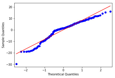
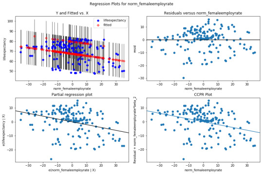
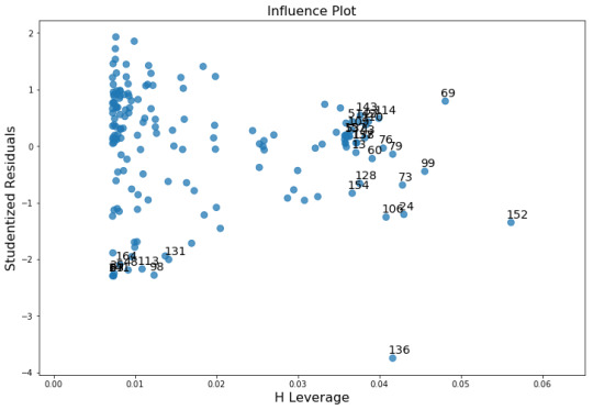
There is a non-linear relationship at the outer quartiles.  There is a poor linear fit in the residuals and an outlier (almost 4 standard deveations from the mean) that should be removed from the analysis and re-run.  

[jcvallier]

Regression Modeling - Week 3

For this week I used the Gapminder data set variables life expectancy and empoyment rate.  I used a regression analysis to determine if employment rate is associated with life expectancy.   

I adjusted the employment rate variable by subtracting each observation by the mean of approximately 58.99.  This normalized the variable by centering the mean to zero.  

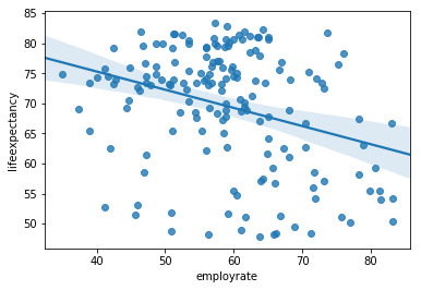
The regression analysis gave me a p-value of zero and a formula of y=-.03x+69.54. The r squared is .10

This means that for every 1 point increase in employment rate decreases life expectancy by .03.  

This model has a negative trend showing employment rate to be significant, but I would not consider this to be a robust model, as the r-squared is a weak score of.10 and the residuals are not linear.  

Program and Output:

import warnings import statsmodels.api as sm import statsmodels.formula.api as smf import seaborn as sns warnings.filterwarnings("ignore")

df2 = df1[['lifeexpectancy','employrate']] df2['norm_employrate'] = df2['employrate'] - df2['employrate'].mean() df2['norm_employrate'].mean() df2['trans_employrate'] = np.exp(df2['employrate'])

modelname = smf.ols(formula='lifeexpectancy ~ norm_employrate', data = df2).fit() print(modelname.summary())

print('average life exp:' , df2['lifeexpectancy'].mean()) print('average employ rate:' , df2['employrate'].mean())

sns.regplot(x='employrate',y='lifeexpectancy', data=df2)                            OLS Regression Results                             ============================================================================== Dep. Variable:         lifeexpectancy   R-squared:                       0.099 Model:                            OLS   Adj. R-squared:                  0.093 Method:                 Least Squares   F-statistic:                     17.94 Date:                Sun, 08 Oct 2017   Prob (F-statistic):           3.79e-05 Time:                        15:24:51   Log-Likelihood:                -607.59 No. Observations:                 166   AIC:                             1219. Df Residuals:                     164   BIC:                             1225. Df Model:                           1                                         Covariance Type:            nonrobust                                         ===================================================================================                      coef    std err          t      P>|t|      [0.025      0.975] ----------------------------------------------------------------------------------- Intercept          69.5456      0.734     94.694      0.000      68.095      70.996 norm_employrate    -0.3021      0.071     -4.235      0.000      -0.443      -0.161 ============================================================================== Omnibus:                       11.183   Durbin-Watson:                   1.772 Prob(Omnibus):                  0.004   Jarque-Bera (JB):               12.051 Skew:                          -0.639   Prob(JB):                      0.00242 Kurtosis:                       2.669   Cond. No.                         10.3 ==============================================================================

Warnings: [1] Standard Errors assume that the covariance matrix of the errors is correctly specified. average life exp: 69.54557228915664 average employ rate: 58.9879518766265

average norm employ rate: 9.16000876220852e-15

[jcvallier]

Regression - Week 1

Source: Gapminder.com

 Sample

We have decided to include the following entities:

192 UN members (as of April 2008)

51 other entities listed in the “List of countries” in Wikipedia (2008-05-13). These include the     Vatican, dependent territories, special entities and disputed territories.     We have excluded the two “sub-dependencies” Ascension Island and Tristan     da Cunha, although they are listed by Wikipedia.

4 French overseas territories (Guadeloupe, Martinique,     Reunion and French Guyana), although they are considered an integral part     of France

10 former states

2 ad-hoc areas: “Serbia excluding Kosovo” and “the     Channel Islands”. The latter is the collective name of the two dependent     territories Guernsey and Jersey.

In spetember 2012 we added the new UN state “South     Sudan” to our country list. The new number of UN members are hence 193.     This gives a total of 193+51+4+10+2=260 countries and     territories. Our goal is to have data for all these entities for at least     two indicators (one of them being population), from 1800 onwards. However,     most indicators will only have data for a selection of these entities.

Procedure

The main purpose of this observational data is to produce graphical presentations that display the magnitude of health and wealth disparities in the contemporary world. Therefore, we have also included rough estimates for countries and territories for which reliable data was not available for 2006. These estimates can only be taken as an indication of the order of magnitude for the indicator. Furthermore, we have not been able to make sure that every single observation is based on the best estimates available. Hence we discourage the use of this data set for statistical analysis and advise those who require more exact data to investigate the available data more carefully and look for additional sources, when appropriate.

Variables

The main analysis performed used income per person to predict employment rate.  The income per person comes from 2010 Gross Domestic Product per capita in constant 2000 US$. The inflation but not the differences in the cost of living between countries has been taken into account.  Employment rate is 2007 total employees age 15+ (% of population) Percentage of total population, age above 15, that has been employed during the given year.

[jcvallier]

Data Analysis Tools- Week 4

This week we have learned about moderators and how they act as a third variable that affects the strength of the relationship between a dependent and independent variable.  

This week I picked income per person to explain female employment rate as my two variables.  I also chose developed countries and non-developed countries as my moderator.

When looking at the income per person and female employment rate, I have an r  square of 0.00.  

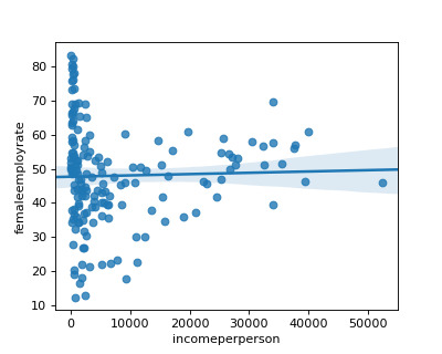
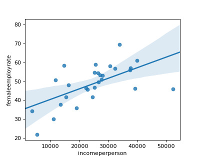
Now, I introduce the moderator of developed countries to find if income per person can explain the female employment rate in this subgroup.

I found that in developed countries, there is a positive relationship between higher income per person and higher female employment rate. This is reflected in the higher r square score of 0.37.

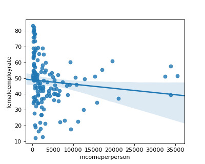
I found that in non developed countries, there is a negative relationship between income per person and higher female employment rate. But, this is reflected in the lower r square score of 0.13.

Code:

#import libraries import pandas as pd from scipy.stats import pearsonr import matplotlib.pyplot as plt import seaborn as sns

# import data data = pd.read_csv('GapminderData.csv')

# select the variables of interest df1 = data[['country','lifeexpectancy','employrate','femaleemployrate','DevelCountry','incomeperperson']]

# new variable  - earningpower (lifeexpectancy * incomeperperson) - this is not an average lifetime income but an indication of earning power potential over ones lifetime

df1['earningpower'] = df1['lifeexpectancy'] * df1['incomeperperson']

# new variable - unemployment (100 - 'employrate') - this is the percentage of the population who does not hold a job

df1['unemployment'] = 100 - df1['employrate']

# new variable - femaleunemployment (100 - 'femaleemployrate') - this is the percentage of females who does not hold a job

df1['femaleunemployment'] = 100 - df1['femaleemployrate']

# how many NAs do we have in employrate

print(df1['employrate'].value_counts(dropna=False))

# drop countries that does not have employrate variable

df1 = df1[pd.notnull(df1['employrate'])]

# did we remove the NAs in employrate variable?

print(df1['employrate'].value_counts(dropna=False))

# how many NAs do we have in lifeexpectancy

print(df1['lifeexpectancy'].value_counts(dropna=False))

# drop contries that have NAs in lifeexpenctancy

df1 = df1[pd.notnull(df1['lifeexpectancy'])]

# did we remove the NAs in lifeexpectancy

print(df1['lifeexpectancy'].value_counts(dropna=False))

reg = sns.regplot(x='incomeperperson',y='femaleemployrate',data = df1)

fig = reg.get_figure() fig.savefig('ploy.png')

# run scipy stats pearson correlation (R correlation, P Value) x = df1['incomeperperson'] y = df1['femaleemployrate']

pearsonr(x,y)

0.02836*0.02836

df2 = df1[df1['DevelCountry']==1] df3 = df1[df1['DevelCountry']==0]

reg1 = sns.regplot(x='incomeperperson',y='femaleemployrate',data = df2)

fig = reg1.get_figure() fig.savefig('ploy1.png')

x = df2['incomeperperson']

y = df2['femaleemployrate']

pearsonr(x,y)

0.60528 * 0.60528

reg2 = sns.regplot(x='incomeperperson',y='femaleemployrate',data = df3)

fig = reg2.get_figure() fig.savefig('ploy2.png')

x = df3['incomeperperson'] y = df3['femaleemployrate']

pearsonr(x,y)

-0.11386 * -0.11386

[jcvallier]

Data Analysis Tools - Week 3

This week I used life expectancy to explain the employment rate in developed countries vs non-developed countries.

My Code:

#import libraries import pandas as pd from scipy.stats import pearsonr import seaborn as sns

#import data data = pd.read_csv('GapminderData.csv')

#Visualization of life expectancy and employment rate sns.regplot(x='lifeexpectancy',y='employrate', data=data)

# run scipy stats pearson correlation (R correlation, P Value) x = data['lifeexpectancy'] y = data['employrate']

pearsonr(x,y)

# life expectancy to explain employment rate in developed countries dev = data[data['DevelCountry'] == 1] sns.regplot(x='lifeexpectancy',y='employrate', data=dev)

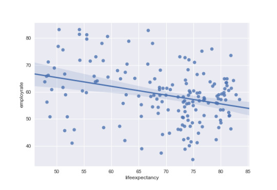
# run scipy stats pearson correlation (R correlation, P Value) x = dev['lifeexpectancy'] y = dev['employrate']

pearsonr(x,y)

rsquare = (-.3140)*(-.3140)

# life expectancy to explain employment rate in developed countries dev = data[data['DevelCountry'] == 1]

regfig2 = sns.regplot(x='lifeexpectancy',y='employrate', data=dev)

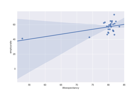
# run scipy stats pearson correlation (R correlation, P Value) x = dev['lifeexpectancy'] y = dev['employrate']

pearsonr(x,y)

rsquare = (.4872)*(.4872)

# life expectancy to explain employment rate in non-developed countries nondev = data[data['DevelCountry'] == 0] regfig3 = sns.regplot(x='lifeexpectancy',y='employrate', data=nondev)

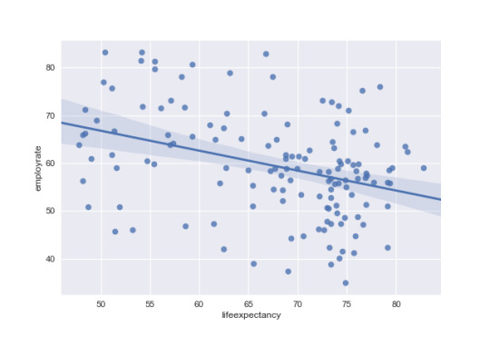
# run scipy stats pearson correlation (R correlation, P Value) x = nondev['lifeexpectancy'] y = nondev['employrate']

pearsonr(x,y)

rsquare = (-.3648)*(-.3648)

## Summary of Correlation (Developed vs. Non-Developed Countries)

Looking at all countries the R correlation life expectancy has a negative relationship with employment rate of -0.31 and a p value of less than .05.  This means there is a significat relationship where employment rate decreases as life expectancy increases.  There is also an r square of .099 which means life expectancy can explain approxamatly 10% of the variance.  

Then, Looking at developed countries the R correlation life expectancy has a positive relationship with employment rate of 0.49 and a p value of less than .05.  This means there is a significat relationship where employment rate increaes as life expectancy increases.  There is also an r square of .237 which means life expectancy can explain approxamatly 24% of the variance.

Finally, Looking at non-developed countries the R correlation life expectancy has a negative relationship with employment rate of -0.36 and a p value of less than .05.  This means there is a significat relationship where employment rate decreases as life expectancy increases.  There is also an r square of 0.133 which means life expectancy can explain approxamatly 13% of the variance.

[jcvallier]

Data Analysis Tools - Week 2

Model Interpretation for Chi-Square Tests:

For this test I needed to create two new variables perc_group & perc_lifeexp. Where perc_group is three groups( by percentile 0-33%,34-66%,67-100%) from income per person variable.  Perc_lifeexp is three groups (by percentile 0-33%,34-66%,67-100%) from life expectancy variable.

When examining the association between life expectancy and income per person, a chi-square test of independence revealed that higher income percentile have longer life spans. The top income percentile has a life expectancy of 76-83 years old, 83% of the time.  The middle income percentile has a life expectancy of 68-75, 63% of the time . The bottom life expectancy is 47-67, 78% of the time. X2 =136.9, 2 df, p=1.285e-28.

Model Interpretation for post hoc Chi-Square Test results:

A Chi Square test of independence revealed the null hypothsysis can be rejected between life expectancy and income per person.  

Post hoc comparisons of rate adjusted for the Bonferroni adjustment is .05/3  = .02. When comparing this with the pvalue = 1.285e-28 this post hoc evaulation confirms we are correct in rejecting the null hypothsysis 

perc_lifeexp   1   2   3 perc_group               1             46  10   1 2              8  35  11 3              1  11  43 perc_lifeexp         1         2         3 perc_group                                 1             0.836364  0.178571  0.018182 2             0.145455  0.625000  0.200000 3             0.018182  0.196429  0.781818 Chi Square value, p value, excpected counts (136.92436043046089, 1.2852905779637279e-28, 4, array([[ 18.88554217,  19.22891566,  18.88554217],       [ 17.89156627,  18.21686747,  17.89156627],       [ 18.22289157,  18.55421687,  18.22289157]]))

Code

import pandas as pd

# import data data = pd.read_csv('GapminderData.csv')

# select the variables of interest df1 = data[['country','lifeexpectancy','employrate','femaleemployrate','DevelCountry','incomeperperson','perc_group','perc_lifeexp']]

# new variable  - earningpower (lifeexpectancy * incomeperperson) - this is not an average lifetime income but an indication of earning power potential over ones lifetime

df1['earningpower'] = df1['lifeexpectancy'] * df1['incomeperperson']

# new variable - unemployment (100 - 'employrate') - this is the percentage of the population who does not hold a job

df1['unemployment'] = 100 - df1['employrate']

# new variable - femaleunemployment (100 - 'femaleemployrate') - this is the percentage of females who does not hold a job

df1['femaleunemployment'] = 100 - df1['femaleemployrate']

# how many NAs do we have in employrate

print(df1['employrate'].value_counts(dropna=False))

# drop countries that does not have employrate variable

df1 = df1[pd.notnull(df1['employrate'])]

# did we remove the NAs in employrate variable?

print(df1['employrate'].value_counts(dropna=False))

# how many NAs do we have in lifeexpectancy

print(df1['lifeexpectancy'].value_counts(dropna=False))

# drop contries that have NAs in lifeexpenctancy

df1 = df1[pd.notnull(df1['lifeexpectancy'])]

# did we remove the NAs in lifeexpectancy

print(df1['lifeexpectancy'].value_counts(dropna=False))

df1.dropna(inplace=True)

sht3.range('A1').expand('table').value = df1

print(df1['lifeexpectancy'].max()) print(df1['lifeexpectancy'].min())

CROSS = pd.crosstab(df1['perc_group'],df1['perc_lifeexp'])

print(CROSS)

#%%

colsum = CROSS.sum(axis=0) colpct = CROSS/colsum print(colpct)

#%%

print('Chi Square value, p value, ecpected counts') gchi1 = sci.stats.chi2_contingency(CROSS) print(chi1)

[jcvallier]

Data Analysis Tools - Week 1

(gapminder dataset)

Model Interpretation for ANOVA:

Using income per person variable, I put the bottom 1/3, middle 1/3, and top 1/3 percentile into a 3,2,1 values, respectively.  This variable is the income percentile group or perc_group.

When examining the association between employment rate and income percentile group, an Analysis of Variance (ANOVA) there is a significant difference between the top, middle, and bottom, with the mean and standard deviation for top percentile is a Mean=57.34% /  s.d. ±7.51%, for the middle percentile is a Mean=55.22% /  s.d. ±9.46%, and bottom percentile is a Mean=64.39% / s.d. ±11.53%, F score=13.66, p value = 3.27e-06.  Since the p value is less than 0.05 there is a significant difference between the means and we reject the null hypothesis.

The degrees of freedom can be found in the OLS table as the DF model and DF residuals 2 and 163, respectively. 

 OLS Regression Results                             ============================================================================== Dep. Variable:             employrate   R-squared:                       0.144 Model:                            OLS   Adj. R-squared:                  0.133 Method:                 Least Squares   F-statistic:                     13.66 Date:                Mon, 04 Sep 2017   Prob (F-statistic):           3.27e-06 Time:                        23:47:31   Log-Likelihood:                -609.75 No. Observations:                 166   AIC:                             1226. Df Residuals:                     163   BIC:                             1235. Df Model:                           2                                         Covariance Type:            nonrobust                                         ======================================================================================                         coef    std err          t      P>|t|      [95.0% Conf. Int.] -------------------------------------------------------------------------------------- Intercept             57.3386      1.274     45.020      0.000        54.824    59.854 C(perc_group)[T.2]    -2.1145      1.826     -1.158      0.249        -5.720     1.491 C(perc_group)[T.3]     7.0541      1.817      3.881      0.000         3.465    10.643 ============================================================================== Omnibus:                        0.415   Durbin-Watson:                   1.951 Prob(Omnibus):                  0.813   Jarque-Bera (JB):                0.460 Skew:                          -0.118   Prob(JB):                        0.794 Kurtosis:                       2.894   Cond. No.                         3.68 ==============================================================================

Warnings: [1] Standard Errors assume that the covariance matrix of the errors is correctly specified.

Model Interpretation of post hoc ANOVA results:

ANOVA analysis p value was significant, but to determine which of the means are significantly different I ran a Post hoc test, using ‘Tukey Honest Sigificant Difference’.  

Multiple Comparison of Means - Tukey HSD,FWER=0.05 ============================================ group1 group2 meandiff lower   upper  reject --------------------------------------------  1      2    -2.1145  -6.434  2.2049 False  1      3     7.0541  2.7549 11.3534  True  2      3     9.1687  4.8112 13.5261  True --------------------------------------------

When compared with employment rate, there is a difference between top and bottom income percentiles.  There is also a difference between middle and bottom income percentiles.   

Related Code:

import pandas as pd

data = pd.read_csv('GapminderData.csv')

# select the variables of interest df1 = data[['country','lifeexpectancy','employrate','femaleemployrate','DevelCountry','incomeperperson','perc_group']]

# new variable  - earningpower (lifeexpectancy * incomeperperson) - this is not an average lifetime income but an indication of earning power potential over ones lifetime

df1['earningpower'] = df1['lifeexpectancy'] * df1['incomeperperson']

# new variable - unemployment (100 - 'employrate') - this is the percentage of the population who does not hold a job

df1['unemployment'] = 100 - df1['employrate']

# new variable - femaleunemployment (100 - 'femaleemployrate') - this is the percentage of females who does not hold a job

df1['femaleunemployment'] = 100 - df1['femaleemployrate']

# how many NAs do we have in employrate

print(df1['employrate'].value_counts(dropna=False))

# drop countries that does not have employrate variable

df1 = df1[pd.notnull(df1['employrate'])]

# did we remove the NAs in employrate variable?

print(df1['employrate'].value_counts(dropna=False))

# how many NAs do we have in lifeexpectancy

print(df1['lifeexpectancy'].value_counts(dropna=False))

# drop contries that have NAs in lifeexpenctancy

df1 = df1[pd.notnull(df1['lifeexpectancy'])]

# did we remove the NAs in lifeexpectancy

print(df1['lifeexpectancy'].value_counts(dropna=False))

df1.dropna(inplace=True)

#%%

df4 = df1[['employrate','perc_group']]

#%%

import statsmodels.formula.api as smf import statsmodels.stats.multicomp as multi

model = smf.ols(formula='employrate ~ C(perc_group)',data=df4) results = model.fit() print(results.summary())

#%%

df5=df4.groupby('perc_group').mean() df6=df4.groupby('perc_group').std()

print(df5,df6)

#%%

mc = multi.MultiComparison(df4['employrate'],df4['perc_group']) result2 = mc.tukeyhsd() print(result2.summary())

[jcvallier]

Data Management and Visualization - Week 4

I have selected the following variables to visualize (python: .describe() function):

     lifeexpectancy  employrate  femaleemployrate  DevelCountry  \ count      166.000000  166.000000        166.000000    166.000000   mean        69.545572   58.987952         47.963855      0.168675   std          9.936253   10.327332         14.618138      0.375597   min         47.794000   34.900002         12.400000      0.000000   25%         62.725000   51.575001         39.250001      0.000000   50%         73.129000   58.850000         48.450001      0.000000   75%         76.844750   64.975000         56.150001      0.000000   max         83.394000   83.199997         83.300003      1.000000  

      incomeperperson  earningpower  unemployment  femaleunemployment   count       166.000000  1.660000e+02    166.000000          166.000000   mean       7604.543086  5.943488e+05     41.012048           52.036145   std       10812.642619  8.776830e+05     10.327332           14.618138   min         103.775857  5.022440e+03     16.800003           16.699997   25%         609.437746  3.884985e+04     35.025000           43.849999   50%        2507.859649  1.723875e+05     41.150000           51.549999   75%        9209.272098  7.000834e+05     48.424999           60.749999   max       52301.587180  4.182192e+06     65.099998           87.600000  

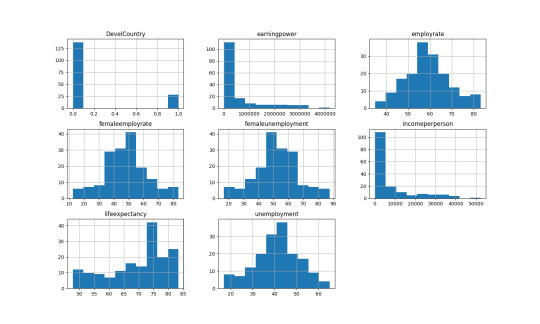
I needed to remove the NAs to perform the histogram analysis.  

The first graph, DevelCountry or ’Developed Countries’, is a categorical variable indicated by 1 or 0.  Here 28 or 16.87% are developed countries out of 166.

 Earningspower and incomperperson is basically the equivalent.   Over 126 of the 166 have income equal to or less than $10,000.  The highest income per person is Luxenberg of $52,301.

Employment rate and unemployment rate are the inverse of each other.  The average employment rate is 59.0% with a standard deviation of 10.3%.     

Female employment rate and female unemployment rate are the inverse of each other, as well.  The average female employment rate is 48.0% with a standard deviation of 14.6%. 

Life expectancy average is 69.5 years with a standard deviation of 9.9 years.

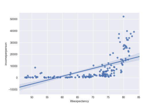
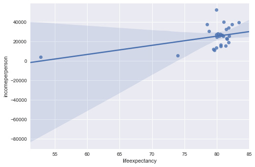
The first bivariate graph is income per person vs. life expectancy as a scatter plot.  This looks like an “L” on its back, where you have countries with similar incomes, but a wide difference in life expectancy. The spike toward the higher end of the plot are related to the developing countries who center around 80 years of life expectancy and much higher income per person. You can confirm this in the second graph, which is only developing countries.  There is a developing country with low income and low life expectancy, South Africa. 

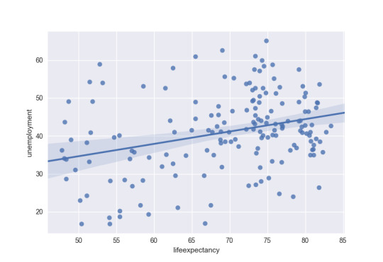
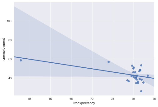
The third and four graph is unemployment and life expectancy.  The data is widely spread around with no real relationship between the two variables.  

[jcvallier]

Data Management and Visualization - Week 3

I added three new varaibles for my week 3 assignment: earningpower, unemployment, and femaleunemployment. 

Earning Power was added to represent potential earnings over ones lifetime and not represented of an average earnings over ones lifetime.  The unemployment rate and female unemployment rate was created as a more intuitive way of viewing the data.

Since my analysis is on how unemployment is associated with life expectancy, I managed these two variables by dropping any ‘NAs’ that existed as I could not infer an average by country, nor would I want to do so.  I left the ‘NAs’ for income per person and earning power as these are more of my secondary variables and not my primary variables.  When I use these columns in any calculation I will manage them according at that time.

Here is my code:

# import libraries import pandas as pdf import numpy as np

# import data data = pd.read_csv('GapminderData.csv')

# select the variables of interest df1 = data[['country','lifeexpectancy','employrate','femaleemployrate','DevelCountry','incomeperperson']]

# new variable  - earningpower (lifeexpectancy * incomeperperson) - this is not an average lifetime income but an indication of earning power potential over ones lifetime

df1['earningpower'] = df1['lifeexpectancy'] * df1['incomeperperson']

# new variable - unemployment (100 - 'employrate') - this is the percentage of the population who does not hold a job

df1['unemployment'] = 100 - df1['employrate']

# new variable - femaleunemployment (100 - 'femaleemployrate') - this is the percentage of females who does not hold a job

df1['femaleunemployment'] = 100 - df1['femaleemployrate']

# how many NAs do we have in employrate

print(df1['employrate'].value_counts(dropna=False))

# drop countries that does not have employrate variable

df1 = df1[pd.notnull(df1['employrate'])]

# did we remove the NAs in employrate variable?

print(df1['employrate'].value_counts(dropna=False))

# how many NAs do we have in lifeexpectancy

print(df1['lifeexpectancy'].value_counts(dropna=False))

# drop contries that have NAs in lifeexpenctancy

df1 = df1[pd.notnull(df1['lifeexpectancy'])]

# did we remove the NAs in lifeexpectancy

print(df1['lifeexpectancy'].value_counts(dropna=False))

# completed managed dataset

print(df1)

Here is my output:

NaN           35 59.900002     3 47.299999     3 58.900002     3 61.500000     3 65.000000     3 53.500000     3 55.900002     3 54.500000     2 60.400002     2 59.000000     2 66.000000     2 58.200001     2 57.500000     2 48.700001     2 56.799999     2 63.799999     2 51.200001     2 61.000000     2 53.400002     2 50.900002     2 83.199997     2 56.000000     2 78.199997     2 51.000000     2 48.599998     2 42.400002     2 70.400002     2 58.400002     2 46.000000     2              .. 57.599998     1 57.200001     1 61.299999     1 54.599998     1 56.400002     1 73.099998     1 79.800003     1 46.200001     1 46.799999     1 41.599998     1 63.200001     1 55.400002     1 44.799999     1 73.199997     1 37.400002     1 41.200001     1 49.599998     1 71.599998     1 44.200001     1 57.099998     1 61.700001     1 62.299999     1 46.400002     1 71.699997     1 57.299999     1 38.900002     1 45.700001     1 55.599998     1 75.199997     1 50.500000     1 Name: employrate, Length: 140, dtype: int64 55.900002    3 59.900002    3 47.299999    3 61.500000    3 53.500000    3 65.000000    3 58.900002    3 48.700001    2 50.900002    2 66.000000    2 58.200001    2 60.400002    2 59.000000    2 54.500000    2 63.799999    2 61.000000    2 51.200001    2 53.400002    2 57.500000    2 56.799999    2 83.199997    2 56.000000    2 59.099998    2 78.199997    2 51.000000    2 48.599998    2 42.400002    2 70.400002    2 58.400002    2 46.000000    2            .. 34.900002    1 41.200001    1 61.299999    1 53.099998    1 54.599998    1 73.099998    1 79.800003    1 46.200001    1 46.799999    1 41.599998    1 63.200001    1 55.400002    1 44.799999    1 73.199997    1 57.599998    1 37.400002    1 49.599998    1 71.599998    1 44.200001    1 57.099998    1 61.700001    1 62.299999    1 46.400002    1 71.699997    1 57.299999    1 38.900002    1 45.700001    1 55.599998    1 75.199997    1 50.500000    1 Name: employrate, Length: 139, dtype: int64 NaN        2 73.979    2 72.974    2 50.239    1 54.675    1 70.349    1 75.850    1 79.158    1 72.477    1 68.846    1 75.901    1 72.150    1 76.640    1 50.411    1 54.116    1 73.235    1 80.934    1 73.339    1 67.185    1 75.181    1 79.120    1 62.095    1 81.126    1 51.093    1 64.986    1 80.557    1 65.437    1 80.414    1 72.640    1 78.531    1          .. 73.403    1 74.044    1 74.941    1 67.017    1 48.196    1 76.835    1 51.088    1 77.005    1 73.131    1 81.097    1 75.620    1 76.652    1 72.231    1 78.371    1 74.156    1 53.183    1 76.072    1 48.673    1 49.025    1 69.042    1 65.493    1 74.825    1 68.823    1 67.852    1 81.618    1 75.632    1 51.610    1 66.618    1 76.848    1 63.125    1 Name: lifeexpectancy, Length: 175, dtype: int64 72.974    2 73.979    2 50.239    1 81.126    1 70.349    1 75.850    1 79.158    1 72.477    1 68.846    1 75.901    1 72.150    1 54.675    1 48.132    1 50.411    1 76.640    1 73.235    1 80.934    1 73.339    1 67.185    1 75.181    1 79.120    1 54.116    1 51.093    1 70.563    1 83.394    1 65.438    1 65.437    1 80.414    1 72.640    1 78.531    1         .. 74.847    1 73.403    1 74.044    1 74.941    1 67.017    1 48.196    1 76.835    1 51.088    1 81.097    1 75.620    1 76.652    1 76.848    1 79.499    1 72.231    1 78.371    1 74.156    1 53.183    1 76.072    1 48.673    1 49.025    1 69.042    1 65.493    1 74.825    1 68.823    1 67.852    1 81.618    1 75.632    1 51.610    1 66.618    1 63.125    1 Name: lifeexpectancy, Length: 174, dtype: int64                    country  lifeexpectancy  employrate  femaleemployrate  \ 0               Afghanistan          48.673   55.700001         25.600000   1                   Albania          76.918   51.400002         42.099998   2                   Algeria          73.131   50.500000         31.700001   4                    Angola          51.093   75.699997         69.400002   6                 Argentina          75.901   58.400002         45.900002   7                   Armenia          74.241   40.099998         34.200001   9                 Australia          81.907   61.500000         54.599998   10                  Austria          80.854   57.099998         49.700001   11               Azerbaijan          70.739   60.900002         56.200001   12                  Bahamas          75.620   66.599998         60.700001   13                  Bahrain          75.057   60.400002         30.200001   14               Bangladesh          68.944   68.099998         53.599998   15                 Barbados          76.835   66.900002         60.299999   16                  Belarus          70.349   53.400002         48.599998   17                  Belgium          80.009   48.599998         41.700001   18                   Belize          76.072   56.799999         38.799999   19                    Benin          56.081   71.599998         58.200001   21                   Bhutan          67.185   58.400002         39.900002   22                  Bolivia          66.618   70.400002         61.599998   23   Bosnia and Herzegovina          75.670   41.200001         34.900002   24                 Botswana          53.183   46.000000         38.700001   25                   Brazil          73.488   64.500000         53.299999   26                   Brunei          78.005   63.799999         55.500000   27                 Bulgaria          73.371   47.299999         42.099998   28             Burkina Faso          55.439   81.300003         75.800003   29                  Burundi          50.411   83.199997         83.300003   30                 Cambodia          63.125   78.900002         73.400002   31                 Cameroon          51.610   59.099998         49.000000   32                   Canada          81.012   63.500000         58.900002   33               Cape Verde          74.156   55.900002         43.599998   ..                      ...             ...         ...               ...   179                   Spain          81.404   52.500000         41.700001   180               Sri Lanka          74.941   55.099998         39.200001   181                   Sudan          61.452   47.299999         27.900000   182                Suriname          70.563   44.700001         30.400000   183               Swaziland          48.718   50.900002         47.099998   184                  Sweden          81.439   60.700001         56.700001   185             Switzerland          82.338   64.300003         57.000000   186                   Syria          75.850   44.799999         16.700001   188              Tajikistan          67.529   54.599998         50.099998   189                Tanzania          58.199   78.199997         76.099998   190                Thailand          74.126   72.000000         65.000000   191             Timor-Leste          62.475   67.300003         54.700001   192                    Togo          57.062   63.900002         48.400002   194     Trinidad and Tobago          70.124   61.500000         50.500000   195                 Tunisia          74.515   41.599998         21.400000   196                  Turkey          73.979   42.799999         21.900000   197            Turkmenistan          64.986   58.500000         53.900002   199                  Uganda          54.116   83.199997         80.000000   200                 Ukraine          68.494   54.400002         49.400002   201    United Arab Emirates          76.546   75.199997         37.299999   202          United Kingdom          80.170   59.299999         53.099998   203           United States          78.531   62.299999         56.000000   204                 Uruguay          77.005   57.500000         46.000000   205              Uzbekistan          68.287   57.500000         52.599998   207               Venezuela          74.402   59.900002         45.799999   208                 Vietnam          75.181   71.000000         67.599998   209      West Bank and Gaza          72.832   32.000000         11.300000   210             Yemen, Rep.          65.493   39.000000         20.299999   211                  Zambia          49.025   61.000000         53.500000   212                Zimbabwe          51.384   66.800003         58.099998       DevelCountry  incomeperperson  earningpower  unemployment  \ 0               0              NaN           NaN     44.299999   1               0      1914.996551  1.472977e+05     48.599998   2               0      2231.993335  1.632279e+05     49.500000   4               0      1381.004268  7.055965e+04     24.300003   6               0     10749.419240  8.158917e+05     41.599998   7               0      1326.741757  9.849863e+04     59.900002   9               1     25249.986060  2.068151e+06     38.500000   10              1     26692.984110  2.158235e+06     42.900002   11              0      2344.896916  1.658757e+05     39.099998   12              0     19630.540550  1.484461e+06     33.400002   13              0     12505.212540  9.386037e+05     39.599998   14              0       558.062877  3.847509e+04     31.900002   15              0      9243.587053  7.102310e+05     33.099998   16              0      2737.670379  1.925924e+05     46.599998   17              1     24496.048260  1.959904e+06     51.400002   18              0      3545.652174  2.697249e+05     43.200001   19              0       377.039699  2.114476e+04     28.400002   21              0      1324.194906  8.896603e+04     41.599998   22              0      1232.794137  8.212628e+04     29.599998   23              0      2183.344867  1.652137e+05     58.799999   24              0      4189.436587  2.228068e+05     54.000000   25              0      4699.411262  3.453503e+05     35.500000   26              0     17092.460000  1.333297e+06     36.200001   27              0      2549.558474  1.870637e+05     52.700001   28              0       276.200413  1.531227e+04     18.699997   29              0       115.305996  5.812691e+03     16.800003   30              0       557.947513  3.522044e+04     21.099998   31              0       713.639303  3.683092e+04     40.900002   32              1     25575.352620  2.071910e+06     36.500000   33              0      1959.844472  1.453342e+05     44.099998   ..            ...              ...           ...           ...   179             1     15461.758370  1.258649e+06     47.500000   180             0      1295.742686  9.710425e+04     44.900002   181             0       523.950151  3.219778e+04     52.700001   182             0      2668.020519  1.882635e+05     55.299999   183             0      1810.230533  8.819081e+04     49.099998   184             1     32292.482980  2.629868e+06     39.299999   185             1     37662.751250  3.101076e+06     35.699997   186             0      1525.780116  1.157304e+05     55.200001   188             0       279.180453  1.885278e+04     45.400002   189             0       456.385712  2.656119e+04     21.800003   190             0      2712.517199  2.010680e+05     28.000000   191             0       369.572954  2.308907e+04     32.699997   192             0       285.224449  1.627548e+04     36.099998   194             0     10480.817200  7.349568e+05     38.500000   195             0      3164.927693  2.358346e+05     58.400002   196             1      5348.597192  3.956839e+05     57.200001   197             0      2062.125152  1.340093e+05     41.500000   199             0       377.421113  2.042452e+04     16.800003   200             0      1036.830725  7.101668e+04     45.599998   201             0     21087.394120  1.614156e+06     24.800003   202             1     28033.489280  2.247445e+06     40.700001   203             1     37491.179520  2.944220e+06     37.700001   204             0      9106.327234  7.012327e+05     42.500000   205             0       952.827261  6.506572e+04     42.500000   207             0      5528.363114  4.113213e+05     40.099998   208             0       722.807559  5.434140e+04     29.000000   209             0              NaN           NaN     68.000000   210             0       610.357367  3.997414e+04     61.000000   211             0       432.226337  2.118990e+04     39.000000   212             0       320.771890  1.648254e+04     33.199997       femaleunemployment   0             74.400000   1             57.900002   2             68.299999   4             30.599998   6             54.099998   7             65.799999   9             45.400002   10            50.299999   11            43.799999   12            39.299999   13            69.799999   14            46.400002   15            39.700001   16            51.400002   17            58.299999   18            61.200001   19            41.799999   21            60.099998   22            38.400002   23            65.099998   24            61.299999   25            46.700001   26            44.500000   27            57.900002   28            24.199997   29            16.699997   30            26.599998   31            51.000000   32            41.099998   33            56.400002   ..                  ...   179           58.299999   180           60.799999   181           72.100000   182           69.600000   183           52.900002   184           43.299999   185           43.000000   186           83.299999   188           49.900002   189           23.900002   190           35.000000   191           45.299999   192           51.599998   194           49.500000   195           78.600000   196           78.100000   197           46.099998   199           20.000000   200           50.599998   201           62.700001   202           46.900002   203           44.000000   204           54.000000   205           47.400002   207           54.200001   208           32.400002   209           88.700000   210           79.700001   211           46.500000   212           41.900002   [176 rows x 9 columns]