friwrite

[friwrite]

Capstone project Draft 3

Preliminary Results

To create the predictor variable it was observed in the different classes their statistical distribution. For example, the PSD of the different tasks(Figure 2) can provide information about the correlation between Movement, Imaginary and Baseline information of all the 10 features extracted. . In previous works of EEG classification is mentioned that correlation between imagery and motor signals can contribute to the performance of a BCI.

  Figure 1. PSD of S1 and 3 tasks.

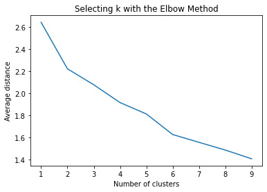
   In the K-means cluster analysis, the variance in the clustering variables that was accounted for by the clusters (r-square) was plotted for each of the nine cluster solutions in an elbow curve to provide guidance for choosing the number of clusters to interpret.  

 Figure 2. Elbow curve of r-square values for the nine cluster solutions

The elbow curve was inconclusive, suggesting that the 2, 4 and 5-cluster solutions might be interpreted. The results below are for an interpretation of the 2-cluster solution.  

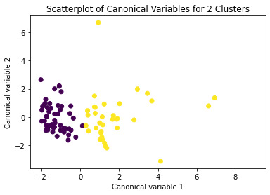
Canonical discriminant analyses was used to reduce the 10 clustering variable down a few variables that accounted for most of the variance in the clustering variables. A scatterplot of the first two canonical variables by cluster (Figure 2 shown below) indicated that the observations in clusters 1 and 2 were densely packed with relatively low within cluster variance, and did not overlap very much with the other clusters. Cluster 2 was generally distinct, but the observations had greater spread suggesting higher within cluster variance. The results of this plot suggest that the best cluster solution may have fewer than 3 clusters, so it will be especially important to also evaluate the cluster solutions with fewer than 4 clusters.  

Figure 3. Plot of the first two canonical variables for the clustering variables by cluster.

 The means on the clustering variables showed that, compared to the other clusters, values in cluster 1 had moderate levels on the clustering variables. They had a relatively low percentage to belong to a inactivity class.

In order to externally validate the clusters, an Analysis of Variance (ANOVA) was conducting to test for significant differences between the clusters on the target variable. A tukey test was used for post hoc comparisons between the clusters. Results indicated significant differences between the clusters on target variable(80.4, p<.0001). The tukey post hoc comparisons showed significant differences between clusters on the target variable, with the exception that clusters 1 and 2 were not significantly different from each other.  Values in cluster 1 had the highest value(mean= -0.0278 , sd=0.81), and cluster 2 had the lowest GPA (mean=-0.2496 , sd=0.19).

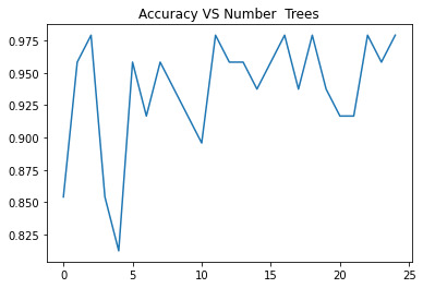
 For the Random Forest analysis the explanatory variables with the highest relative importance scores were  Shannon and the DWT. The accuracy of the random forest was nearly 100% (97.96%) after 25 decision trees (Figure 3)  adding little to the overall accuracy of the model, (that was aprox 94%) and suggesting that interpretation of a single decision tree may be appropriate. 

Note: Each trainning of a Random Forest, increases the accuracy of the model. 

 Figure 4. Random Forest accuracy after 25 decision trees

  Table 1 compares the accuracy for machine learning algorithms of all the available features and pairs of features chosen by their importance for the system. The first column portrays the best percentage of accuracy and corresponds to all the available features. The last column shows the features (Shannon Entropy and Discrete Wavelet Transform pair) that compete with the first column performance. A significant difference in accuracy can be observed depending on the conforming of the selected pairs. The pairs of features which algorithms accuracy compete with the use of all the extracted features are the ones with major relevance for the system

Table 1. MI classification with ML algorithms comparison

[friwrite]

Capstone project Draft 2

Methods.

 The database selected for their support information and size was the Physionet Motor-Imagery dataset. The complete database consisting of 1500 recordings of 1- 2 minutes was obtained from 109 volunteers on 64 EEG channels using the BCI2000 system. Each subject performed 14 experimental runs, with the following characteristics: two one-minute baseline runs (one with eyes open, one with eyes closed) and three experimental runs of two minutes of each of the following four tasks: 1) Open and close the left or right fist 2) Imagine opening or closing the left or right fist 3) Open and close both fists or both feet 4) Imagine opening and closing both fists or both feet.

For the present work, not the full database was employed, only a sub-set of 10 experimental subjects because an A 10% subject size can represent the information. The selection of the size was made taking into consideration previous studies that demonstrate feature correlation with a small sample and to lower the computational cost.  Also, the sub-set is composed of  10 experimental subjects that contain 12 trials each. 3 trials correspond to the performance of the movement,  3 trials to the imagination of the movement, and six trials to a baseline (3 for eyes open and 3 for eyes closed), giving a total of 120 trials.

 In this work, features were extracted and selected based on their association with the cerebral motor region to facilitate the distinction of movement (real or imaginary) and inactivity. The features were extracted for the Fc3 channel, this channel was considered due to its location in the 20-10 electrode positioning system and also its in a region associated with motor activity. It was extracted 6 power bands  Delta, Theta, Alpha, Beta, Gama, and Mu (an alphoid associated with motor events).

And time-domain features that reflected the randomness of the signals and could be helpful to distinguish between movement and inactivity, that was the following: Spectral Power Density (PSD) that it’s a rate witch motor unities are triggered, Shannon Entropy a measure of uncertainty, and a representation of certain signal information, Spectral Entropy a measure of power distribution and Discrete Wavelet Transform (DWT) that is the decomposition of the signal in basic functions by contraction or expansions of their equations.

 A K-means cluster analysis was conducted to identify underlying subgroups of  variables based on their similarity of responses on 10 variables that represent characteristics that could have an impact on movement in EEG signals.

All clustering variables were standardized to have a mean of 0 and a standard deviation of 1.

Data were randomly split into a training set that included 70% of the observations (N=84) and a test set that included 30% of the observations (N=36). A series of k-means cluster analyses were conducted on the training data specifying k=1-9 clusters, using Euclidean distance.

Also, a Random Forest analysis was performed to evaluate the importance of a series of explanatory variables in predicting  a binary, categorical response variable, that in the present is called represented by the inactivity or the movement. The 10 EEG explanatory variables were included as a possible contributors to random forest evaluation of the movement condition These features, including power bands and time-domain features,  and a binary, categorical response variable, to classify between inactivity or movement. PSD, 2 types of Entropy, a Discrete Wavelet and 6 Power Bands calculations. The data was split into train 60% and test in 40%.

[friwrite]

Capstone Project Draft 1

Title:  EEG motor/imagery feature comparision and ranking

Introduction: The purpose of this study is to identify the pair of features that are most relevant for an EEG Motor/Imaginary signal system, between some time-domain features (like PSD), and power bands In EEG, Movement Imaginary (MI)  has been a fundamental part of the development of assistive rehabilitation technologies such as BCI. These assistive technologies are composed of devices, products, or pieces of equipment used to increase, maintain, or improve the independence of people with different levels of disability. This feature rank could lead to improving the feature extraction process and increase the level of accuracy in a motor/imagery signal classification in the future.

[friwrite]

K-means Cluster

Task

A k-means cluster analysis was conducted to identify underlying subgroups of adolescents based on their similarity of responses on 10 variables that represent characteristics that could have an impact on movement in EEG signals.

Data

The data was a sample of 10 subjects and 3 trials of upper limb movement taken from the Physionet Motor/Imagery data set.https://physionet.org/content/eegmmidb/1.0.0/

Results

 Clustering variables including power bands and time-domain features,  and a binary, categorical response variable, to classify between inactivity or movement. All clustering variables were standardized to have a mean of 0 and a standard deviation of 1.

Data were randomly split into a training set that included 70% of the observations (N=84) and a test set that included 30% of the observations (N=36). A series of k-means cluster analyses were conducted on the training data specifying k=1-9 clusters, using Euclidean distance. The variance in the clustering variables that was accounted for by the clusters (r-square) was plotted for each of the nine cluster solutions in an elbow curve to provide guidance for choosing the number of clusters to interpret.  

Figure 1. Elbow curve of r-square values for the nine cluster solutions

The elbow curve was inconclusive, suggesting that the 2, 4 and 5-cluster solutions might be interpreted. The results below are for an interpretation of the 2-cluster solution.  

Canonical discriminant analyses was used to reduce the 10 clustering variable down a few variables that accounted for most of the variance in the clustering variables. A scatterplot of the first two canonical variables by cluster (Figure 2 shown below) indicated that the observations in clusters 1 and 2 were densely packed with relatively low within cluster variance, and did not overlap very much with the other clusters. Cluster 2 was generally distinct, but the observations had greater spread suggesting higher within cluster variance. The results of this plot suggest that the best cluster solution may have fewer than 3 clusters, so it will be especially important to also evaluate the cluster solutions with fewer than 4 clusters.  

Figure 2. Plot of the first two canonical variables for the clustering variables by cluster.  

The means on the clustering variables showed that, compared to the other clusters, values in cluster 1 had moderate levels on the clustering variables. They had a relatively low percentage to elong to a inactivity class.

In order to externally validate the clusters, an Analysis of Variance (ANOVA) was conducting to test for significant differences between the clusters on the target variable. A tukey test was used for post hoc comparisons between the clusters. Results indicated significant differences between the clusters on target variable(80.4, p<.0001). The tukey post hoc comparisons showed significant differences between clusters on the target variable, with the exception that clusters 1 and 2 were not significantly different from each other.  Values in cluster 1 had the highest value(mean= -0.0278 , sd=0.81), and cluster 2 had the lowest GPA (mean=-0.2496 , sd=0.19).

Code

data = pd.read_csv("eegclass.csv")

#upper-case all DataFrame column names data.columns = map(str.upper, data.columns)

# Data Management

data_clean = data.dropna()

# subset clustering variables cluster=data_clean[['PSD','SHANON','SPECTRAL','DWT', 'DELTA','TETA',                         'ALFA','BETA', 'GAMA','MU']] cluster.describe()

# standardize clustering variables to have mean=0 and sd=1 clustervar=cluster.copy() clustervar['PSD']=preprocessing.scale(clustervar['PSD'].astype('float64')) clustervar['SHANON']=preprocessing.scale(clustervar['SHANON'].astype('float64')) clustervar['SPECTRAL']=preprocessing.scale(clustervar['SPECTRAL'].astype('float64')) clustervar['DWT']=preprocessing.scale(clustervar['DWT'].astype('float64')) clustervar['DELTA']=preprocessing.scale(clustervar['DELTA'].astype('float64')) clustervar['TETA']=preprocessing.scale(clustervar['TETA'].astype('float64')) clustervar['ALFA']=preprocessing.scale(clustervar['ALFA'].astype('float64')) clustervar['BETA']=preprocessing.scale(clustervar['BETA'].astype('float64')) clustervar['GAMA']=preprocessing.scale(clustervar['GAMA'].astype('float64')) clustervar['MU']=preprocessing.scale(clustervar['MU'].astype('float64'))

# split data into train and test sets clus_train, clus_test = train_test_split(clustervar, test_size=.3, random_state=123)

# k-means cluster analysis for 1-9 clusters                                                           from scipy.spatial.distance import cdist clusters=range(1,10) meandist=[]

for k in clusters:    model=KMeans(n_clusters=k)    model.fit(clus_train)    clusassign=model.predict(clus_train)    meandist.append(sum(np.min(cdist(clus_train, model.cluster_centers_, 'euclidean'), axis=1))    / clus_train.shape[0])

""" Plot average distance from observations from the cluster centroid to use the Elbow Method to identify number of clusters to choose """

plt.plot(clusters, meandist) plt.xlabel('Number of clusters') plt.ylabel('Average distance') plt.title('Selecting k with the Elbow Method')

# Interpret 2 cluster solution model3=KMeans(n_clusters=2) model3.fit(clus_train) clusassign=model3.predict(clus_train) # plot clusters

from sklearn.decomposition import PCA pca_2 = PCA(2) plot_columns = pca_2.fit_transform(clus_train) plt.scatter(x=plot_columns[:,0], y=plot_columns[:,1], c=model3.labels_,) plt.xlabel('Canonical variable 1') plt.ylabel('Canonical variable 2') plt.title('Scatterplot of Canonical Variables for 2 Clusters') plt.show()

""" BEGIN multiple steps to merge cluster assignment with clustering variables to examine cluster variable means by cluster """ # create a unique identifier variable from the index for the # cluster training data to merge with the cluster assignment variable clus_train.reset_index(level=0, inplace=True) # create a list that has the new index variable cluslist=list(clus_train['index']) # create a list of cluster assignments labels=list(model3.labels_) # combine index variable list with cluster assignment list into a dictionary newlist=dict(zip(cluslist, labels)) newlist # convert newlist dictionary to a dataframe newclus=DataFrame.from_dict(newlist, orient='index') newclus # rename the cluster assignment column newclus.columns = ['cluster']

# now do the same for the cluster assignment variable # create a unique identifier variable from the index for the # cluster assignment dataframe # to merge with cluster training data newclus.reset_index(level=0, inplace=True) # merge the cluster assignment dataframe with the cluster training variable dataframe # by the index variable merged_train=pd.merge(clus_train, newclus, on='index') merged_train.head(n=100) # cluster frequencies merged_train.cluster.value_counts()

""" END multiple steps to merge cluster assignment with clustering variables to examine cluster variable means by cluster """

# FINALLY calculate clustering variable means by cluster clustergrp = merged_train.groupby('cluster').mean() print ("Clustering variable means by cluster") print(clustergrp)

# validate clusters in training data by examining cluster differences in GPA using ANOVA # first have to merge GPA with clustering variables and cluster assignment data gpa_data=data_clean['LABEL'] # split GPA data into train and test sets gpa_train, gpa_test = train_test_split(gpa_data, test_size=.3, random_state=123) gpa_train1=pd.DataFrame(gpa_train) gpa_train1.reset_index(level=0, inplace=True) merged_train_all=pd.merge(gpa_train1, merged_train, on='index') sub1 = merged_train_all[['LABEL', 'cluster']].dropna()

import statsmodels.formula.api as smf import statsmodels.stats.multicomp as multi

gpamod = smf.ols(formula='LABEL ~ C(cluster)', data=sub1).fit() print (gpamod.summary())

print ('means for Label by cluster') m1= sub1.groupby('cluster').mean() print (m1)

print ('standard deviations for Label by cluster') m2= sub1.groupby('cluster').std() print (m2)

mc1 = multi.MultiComparison(sub1['LABEL'], sub1['cluster']) res1 = mc1.tukeyhsd() print(res1.summary())

[friwrite]

Lasso Regression

Task

A lasso regression analysis was conducted to identify a subset of variables from a pool of 10 categorical and quantitative predictor variables that best predicted a quantitative response variable measuring movement and inactivity conditions  in eeg signals. Categorical predictors  including power bands and time-domain features,  and a binary, categorical response variable, to classify between inactivity or movement.  All predictor variables were standardized to have a mean of zero and a standard deviation of one.

Data

The data was a sample of 10 subjects and 3 trials of upper limb movement taken from the Physionet Motor/Imagery data set.

https://physionet.org/content/eegmmidb/1.0.0/

Results

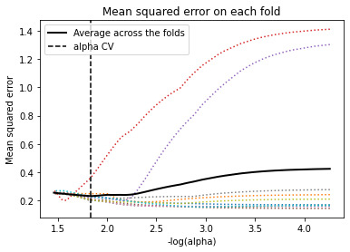
Data were randomly split into a training set that included 70% of the observations (N=84) and a test set that included 30% of the observations (N=36). The least angle regression algorithm with k=10 fold cross validation was used to estimate the lasso regression model in the training set, and the model was validated using the test set. The change in the cross validation average (mean) squared error at each step was used to identify the best subset of predictor variables.

The figure represents the  change in the validation mean square error at each step

The 10 predictor variables were retained in the selected model. During the estimation process, Shannon and DWT  were most strongly associated with MI conditions,  were Shannon is negatively associated with MI conditions.  These 10 variables accounted for 22.9% of the variance MI response variable.

Code

#Data was previously standardize predictors to have mean=0 and sd=1 data = pd.read_csv("eegclasss1.csv")

#select predictor variables and target variable as separate data sets   predictors = data[['PSD','Shanon','Spectral','DWT', 'Delta','Teta',                         'Alfa','Beta', 'Gama','Mu']]

target = data.Label

# split data into train and test sets pred_train, pred_test, tar_train, tar_test = train_test_split(predictors, target,                                                              test_size=.3, random_state=123)

# specify the lasso regression model model=LassoLarsCV(cv=10, precompute=False).fit(pred_train,tar_train)

# print variable names and regression coefficients dict(zip(predictors.columns, model.coef_))

# plot coefficient progression m_log_alphas = -np.log10(model.alphas_) ax = plt.gca() plt.plot(m_log_alphas, model.coef_path_.T) plt.axvline(-np.log10(model.alpha_), linestyle='--', color='k',            label='alpha CV') for idx, feature in enumerate(predictors.columns):    plt.plot(m_log_alphas, list(map(lambda r: r[idx], model.coef_path_.T)), label=feature) plt.legend(loc="upper right", bbox_to_anchor=(1.4, 0.95)) plt.ylabel('Regression Coefficients') plt.xlabel('-log(alpha)') plt.title('Regression Coefficients Progression for Lasso Paths')

# plot mean square error for each fold m_log_alphascv = -np.log10(model.cv_alphas_) plt.figure() plt.plot(m_log_alphascv, model.mse_path_, ':') plt.plot(m_log_alphascv, model.mse_path_.mean(axis=-1), 'k',         label='Average across the folds', linewidth=2) plt.axvline(-np.log10(model.alpha_), linestyle='--', color='k',            label='alpha CV') plt.legend() plt.xlabel('-log(alpha)') plt.ylabel('Mean squared error') plt.title('Mean squared error on each fold')

# MSE from training and test data from sklearn.metrics import mean_squared_error train_error = mean_squared_error(tar_train, model.predict(pred_train)) test_error = mean_squared_error(tar_test, model.predict(pred_test)) print ('training data MSE') print(train_error) print ('test data MSE') print(test_error)

# R-square from training and test data rsquared_train=model.score(pred_train,tar_train) rsquared_test=model.score(pred_test,tar_test) print ('training data R-square') print(rsquared_train) print ('test data R-square') print(rsquared_test)

[friwrite]

Random Forest

Task

Random Forest analysis was performed to evaluate the importance of a series of explanatory variables in predicting  a binary, categorical response variable, that in the present is called represented by the inactivity or the movement. The 10 EEG explanatory variables were included as a possible contributors to random forest evaluation of the movement condition These features,including power bands and time-domian features,  and a binary, categorical response variable, to classify between inactivity or movement. PSD, 2 types of Entropy, a Discrete Wavelet and 6 Power Bands calculations. 

.

Data

The data was a sample of  10 subject and 3 trials of upper limb movement taken from Physionet Motor/Imagery data set.

https://physionet.org/content/eegmmidb/1.0.0/

Results

The explanatory variables with the highest relative importance scores were  Shannon and the DWT. The accuracy of the random forest was nearly 100% (97.96%) after 25 decision trees  adding little to the overall accuracy of the model, (that was aprox 94%) and suggesting that interpretation of a single decision tree may be appropriate. 

Note: Each trainning of a Random Forest, increases the accuracy of the model. 

Code (lines of importance)

#Load the dataset

AH_data = pd.read_csv("eegclass.csv")

data_clean = AH_data.dropna()

data_clean.dtypes data_clean.describe()

#Split into training and testing sets

predictors = data_clean[['PSD','Shanon','Spectral','DWT', 'Delta','Teta',                         'Alfa','Beta', 'Gama','Mu']]

targets = data_clean.Label

pred_train, pred_test, tar_train, tar_test  = train_test_split(predictors, targets, test_size=.4)

pred_train.shape pred_test.shape tar_train.shape tar_test.shape

#Build model on training data from sklearn.ensemble import RandomForestClassifier

classifier=RandomForestClassifier(n_estimators=25) classifier=classifier.fit(pred_train,tar_train)

predictions=classifier.predict(pred_test)

sklearn.metrics.confusion_matrix(tar_test,predictions) sklearn.metrics.accuracy_score(tar_test, predictions)

# fit an Extra Trees model to the data model = ExtraTreesClassifier() model.fit(pred_train,tar_train) # display the relative importance of each attribute print(model.feature_importances_)

""" Running a different number of trees and see the effect of that on the accuracy of the prediction """

trees=range(25) accuracy=np.zeros(25)

for idx in range(len(trees)):   classifier=RandomForestClassifier(n_estimators=idx + 1)   classifier=classifier.fit(pred_train,tar_train)   predictions=classifier.predict(pred_test)   accuracy[idx]=sklearn.metrics.accuracy_score(tar_test, predictions)

#Plotting accuracy vs trees plt.cla() plt.title('Accuracy VS Number Trees'); plt.plot(trees, accuracy)

[friwrite]

Decision Tree

Task

Decision tree analysis was performed to test nonlinear relationships among a series of explanatory variables:10 EEG classification features, including power bands and time-domain features,  and a binary, categorical response variable, to classify between inactivity or movement. 

Data

The data was a sample of 10 subjects and 3 trials of upper limb movement taken from the Physionet Motor/Imagery data set.

https://physionet.org/content/eegmmidb/1.0.0/

Results

The following explanatory variables were included: PSD, 2 types of Entropy and a Discrete Wavelet, and 6 Power Bands calculations as possible contributors to a classification tree model evaluating movement or inactivity (my response variable).

Of the features tested is displayed in the tree the corresponding decision to Mu band. With the following Confusion Matrix:

[19,  1] [ 1, 15]

where the data was split into train 70% and test in 30%. With an accuracy score close to 100%, with a 94.44% of the classification done correctly (because of the size of the sample). 

Code 

#Load the dataset

AH_data = pd.read_csv("eegclass.csv")

data_clean = AH_data.dropna()

data_clean.dtypes data_clean.describe()

""" Modeling and Prediction """ #Split into training and testing sets

predictors = data_clean[['PSD','Shanon','Spectral','DWT', 'Delta','Teta',                         'Alfa','Beta', 'Gama','Mu',]]

targets = data_clean.Label

pred_train, pred_test, tar_train, tar_test  =   train_test_split(predictors, targets, test_size=.3)

pred_train.shape pred_test.shape tar_train.shape tar_test.shape

#Build model on training data classifier=DecisionTreeClassifier() classifier=classifier.fit(pred_train,tar_train)

predictions=classifier.predict(pred_test)

sklearn.metrics.confusion_matrix(tar_test,predictions) sklearn.metrics.accuracy_score(tar_test, predictions)

#Displaying the decision tree from sklearn import tree #Exporting to graphiz and saving in dot archive tree.export_graphviz(classifier, out_file='treeg1.dot') #Ploting tree in python tree.plot_tree(classifier)