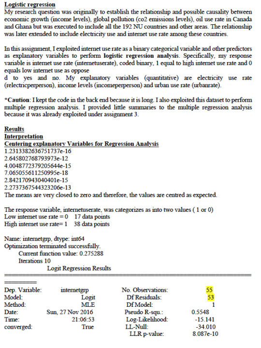
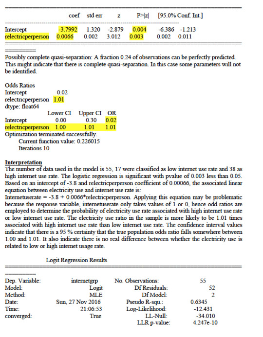
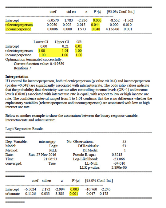
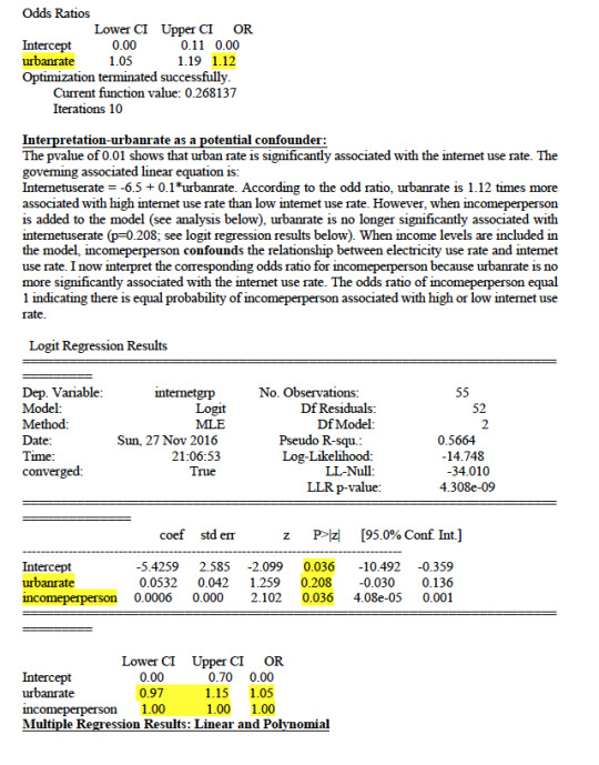
Don't wanna be here? Send us removal request.
Text
Report
Descriptive Statistics
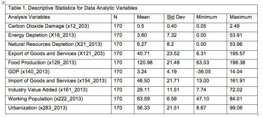
Table 1 shows descriptive statistic for Carbon dioxide emissions calculated in terms of carbon dioxide damage and the quantitative predictors., including one categorical variable (GDP). The mean carbon dioxide damage was 0.5 % of GNI (sd=0.4), with a minimum damage of 0.05 % of GNI and a maximum of 2.49 % of GNI.
Bivariate Analyses
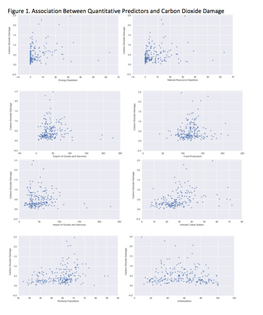
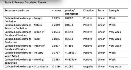
Scatter plots for the association between the carbon dioxide damage response variable and quantitative predictors (Figure 1; Table 2) revealed that carbon dioxide damage increased when industry value added increased (Pearson r=0.38, p<.0001), working population increased (Pearson r=0.34, p<.0001) and energy depletion increased (Pearson r=0.29, p=0.0002). Carbon dioxide damage was not significantly associated with urbanization rate, food production, export of goods and services and import of goods and services.
Lasso Regression Analysis
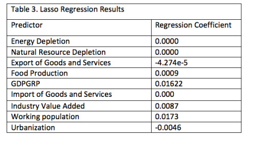
The regression coefficients on Table 3 below show that on applying penalty to the predictor variables; three of the them become zero (Energy depletion, natural resource depletion an import of goods and services), one was almost zero (Export of goods and services). Therefore, using Lasso regression, five of the variables have some effect on carbon dioxide damage (Table 3)
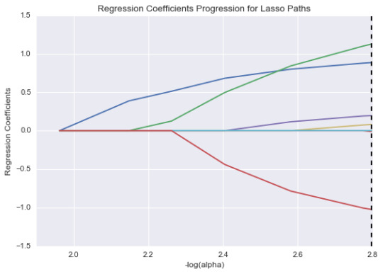
Figure 2 below shows the relative importance of the predictors and the steps in which each variable enters the model. Based on the regression coefficients stated above, the working population and GDP growth were most associated with the carbon dioxide damage, followed by industry value added. Urbanization and export of goods and services were negatively associated with carbon dioxide damage (Table 3; Figure 2).
Figure 2: Regression Coefficient Progression for Lasso Paths
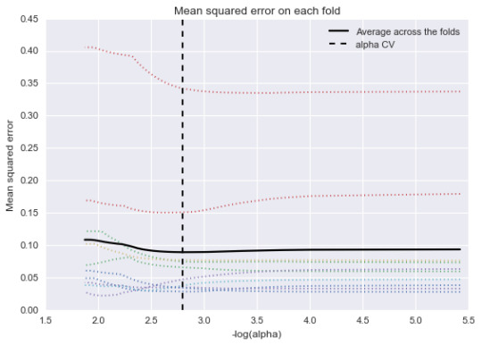
As shown in Figure 3 below, the change in the cross-validation average (mean) squared error at each step was used to identify the best subset of predictor variables. Initially it decreases rapidly and gets to a plateau or levels off at which point adding more predictors doesn’t lead to much reduction in the mean square error. The behavior is expected as model complexity increases
Figure 3: K-Food Mean Square Errors
The mean squared error (MSE) for the test data (MSE=0.16) doubled from the MSE for the training data (MSE=0.08), which suggests that predictive accuracy did decline when the lasso regression algorithm developed on the training data set was applied to predict lead carbon dioxide damage in the test data set.
Also, training data R-square value signifies that 27% variability can be explained for carbon dioxide damage using predictor-variables. Similarly, for test data, the error is 26 % implying that 26 variability of carbon dioxide damage in test data can be explained using predictor variables.
Conclusions/Limitations
This project used lasso regression analysis to identify a subset of world bank related economic indicator variables that best predicted carbon dioxide emissions measured in terms of carbon dioxide damage rate in N=248 world bank countries and regions in 2013. Carbon dioxide damage from 0.05 to 2.49 % of GNI, indicating that there was considerable variability in the amount of carbon dioxide emitted throughout the year.
The Lasso regression analysis indicated that 5 of the 9 developmental related predictor variable were selected in the final model. The strongest predictors of carbon dioxide damage were working population, industry value added and GDP growth. Carbon dioxide damage increased when the working population, industrial activities and GGP growth increased.
There was double increase in the MSE when the training set Lasso regression algorithm was used to predict carbon dioxide damage in the test data set. This suggests that the predictive accuracy of the algorithm may be unstable in future samples, biased and variance in different samples.
The results of this project indicate that controlling population growth rate, transitioning into low carbon economy, energy efficiency and industrial activates based on low carbon input sources are priorities for achieving consistently low carbon dioxide damage (emissions).
Although these three predictors were positively associated with carbon dioxide damage(climate change), the level of association were still weak as the correlation coefficients were all below 0.02 (Table 3). Moreover, neither of these predictors was significantly associated with carbon dioxide damage in the bivariate analyses (Pearson r <0.4; Table 2). However, there are some limitations that should be taken into account when considering changes in the carbon dioxide damage indicator based on the results of this project. First, I analyzed only data from a single year, but changes in the carbon dioxide emissions are ongoing. So, it is important to test this algorithm in carbon dioxide emissions in multiple years to determine whether the algorithm remains relatively biased and unstable despite these ongoing changes. Second, the analysis conducted was limited to the predictor variables available in the dataset. This may lead to misspecification due to the exclusion of important variables from the regression model. There is a large number of economic related factors in the carbon dioxide emission process that could impact climate change, but the current project examined only a few of these factors. It is possible that the factors identified as important predictors of carbon dioxide damage among the set of predictors analyzed in this project are confounded by other factors not considered in this analysis. As a result, these same factors may not emerge as important factors when other factors are taken into consideration. Finally, it appears the dataset was not specifically collected to test the research question. Climate change trends are best observed and evaluated over a time series dataset. Therefore, future efforts to develop a solid predictive algorithm for carbon dioxide emissions should expand the algorithm by adding more developmental indicator predictors to the statistical model, and evaluating the applicability of the algorithm over time series dataset.
0 notes
Text
Methodology
Capstone Project Title:The Association between climate change and economic indicators in World Bank Collated Countries.
Note that I have modified my project title a little bit. I initially choose the title “The Association between climate change and economic indicators in low, medium and high income countries”. The intention was to bin the dataset into 3 subgroups of countries (low, medium and high) and then perform separate statistical analyses on each subgroup. But this will make my sample sizes to be too small for proper statistical analyses. This may introduce more errors into my analyses when I further divide the sub datasets into training and test samples. However, my response variable and predictors remains unchanged
Methods
Sample
The sample (N=248) is from the World Bank Survey on developmental indicators, the main World Bank collection of development Indictors (WDI), compiled from officially-recognized international sources. It presents the most accurate global development data available, and includes national, regional and global estimates. Participants/population (N=198) represented 248 countries and regions of the world with about 168 indicators, including gross domestic product, total employment rate, and estimated HIV prevalence in 2012 and 2013. The sample (N=248) comprises of
Investigating the relationship between economic activities and climate change will help:
a) poor countries to channel their scarce resources to help develop resilience strategies.
b) middle income countries to balance between economic activity and emission control strategic and
c) high income country countries research and develop energy efficiency technologies and shift towards low carbon economy.
Measures
The Co2 damage was measured for each country by multiplying $20 per ton of carbon (the unit damage in 1995 U.S dollars) and the number of tons of carbon emitted.
Predictors included 1) an annual percentage growth of GDP at market price based on constant local currency, 2) export of goods and services and other markets provided to the rest of the world (include the value of merchandise, freight, transport, travel, business and government services 3) import of goods and services and other markets received from the rest of the world (include the value of merchandise, freight, transport, travel, business and government services 4) industry added as a separate net output of the industrial section, 5) annual population growth rate and 6) urbanization growth rate. There are inherent activities in all the predictors that can spur climate change through the emission of more Co2 into the atmosphere.
Analyses
The distributions for the predictors and the carbon dioxide damage response variable were evaluated by performing descriptive statistics for categorical variables and calculating the mean, standard deviation and minimum and maximum values for quantitative variables.
Scatter plots were also examined, and Pearson correlation and Analysis of variance (ANOVA) were used to test bivariate associations between individual predictors and the carbon dioxide damage response variable.
Lasso regression with the least angle regression selection algorithm was used to identify the subset of variables that best predicted carbon dioxide damage. The lasso regression model was estimated on a training data set consisting of a random sample of 60% of the total dataset (N=149), and a test data set included the other 40% of the total dataset (N=99). All predictor variables were standardized to have a mean=0 and standard deviation=1 prior to conducting the lasso regression analysis. Cross validation was performed using k-fold cross validation specifying 10 folds. The change in the cross validation mean squared error rate at each step was used to identify the best subset of predictor variables. Predictive accuracy was assessed by determining the mean squared error rate of the training data prediction algorithm when applied to observations in the test data set.
0 notes
Text
Milestone-1
Capstone Project Title The Association between climate change and economic indicators in low, medium and high income countries. Introduction and motivation to research the project The purpose of this research is to measure the best predictors of a country’s climate change contribution from several economic indicators such as energy consumption, export and import of goods and services, urbanization, industry and gross domestic product (GDP) per capita. We live in an age where the planetary boundaries (such as climate change, ocean acidification, ozone depletion, heavy agriculture loading of nitrogen and phosphorus, overuse of flesh water resources, and biodiversity loss) are getting stressed in addition to increasing poverty in many parts of the world. Global economic activities have pushed the subject of climate change and sustainability to the main stream where individuals, businesses and governments are facing increasing pressure to take action to curve greenhouse gas emissions in order to avoid catastrophic impacts from global warming. The starting point of tackling this problem of the commons is to measure and understand which economic predictors are associated most with climate change (co2 emissions) and thereby developing adaptation and mitigation strategies towards a sustainable future of our planet. I am currently developing new skills in climate change policy, accounting and sustainability reporting. As a native of West Africa and currently living in Canada (North America), I have chosen three groups of countries represented as follows: a) Low income countries: 15 member Ecowas countries located around the equator and within the sub-Saharan region where climate change impact is predicted to be severe. Investigating the relationship between economic activities and climate change will help those countries to channel their scarce resources to help develop resilience strategies. b) Middle income countries: 26 countries including Mexico (North America), who are not spared from climate change impacts. I am hoping this study will add to the growing need for these countries to balance between economic activity and emission control and c) High income country: 26 countries including Canada, which have become a model for other countries in terms of industrialization. I hope this study will contribute to the glowing need to develop energy efficiency technologies and a shift towards renewable energy. Dataset Information I am using the world bank dataset provided by the course. Firstly, the dataset will be cleaned up to include 67 countries representing the 3 income levels (out of the 198 countries provided by the dataset). Secondly, reductant columns from the dataset will be deleted so that the study can be focussed on the indicator variables mentioned. Finally, A series of test including descriptive statistics, scatter plots, Pearson correlation and regression analysis will be conducted to complete the project. In summary, prediction of a moderate to high relationship between economic activities and climate change will move governments of these countries towards a more proactive action on climate and sustainability.
0 notes
Text
K-meansClustering
The GapMinder data set have been consistently used in all my models and assignments.
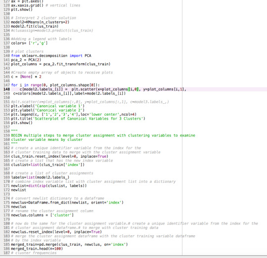
A k-means cluster analysis was conducted to identify underlying subgroups of countries based on their similarity of responses on 14 variables that represent characteristics that could have an impact on country demographics/development. Clustering variables included one binary variable measuring whether or not countries internet use rate is high or low, as well as quantitative variables measuring income levels, armed forces strength, level of pollution in terms of co2 emissions, democratic scores, HIV rate, life expectancy rate, oil use rate, and scales measuring alcohol consumption, breast cancer, female employment, suicide, employment, residential electricity and urbanization rates. All clustering variables were standardized to have a mean of 0 and a standard deviation of 1.
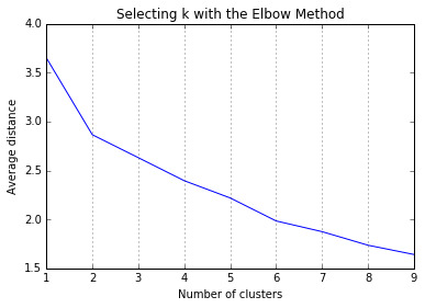
Data were randomly split into a training set that included 70% of the observations (N=38) and a test set that included 30% of the observations (N=17). A series of k-means cluster analyses were conducted on the training data specifying k=1-9 clusters, using Euclidean distance. The variance in the clustering variables that was accounted for by the clusters (r-square) was plotted for each of the nine cluster solutions in an elbow curve to provide guidance for choosing the number of clusters to interpret.
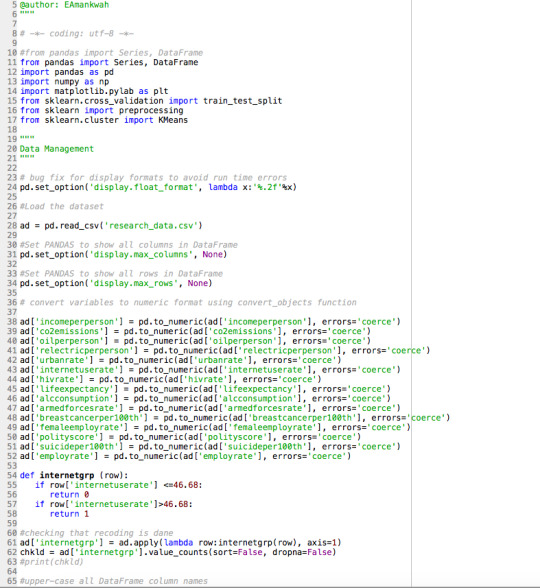
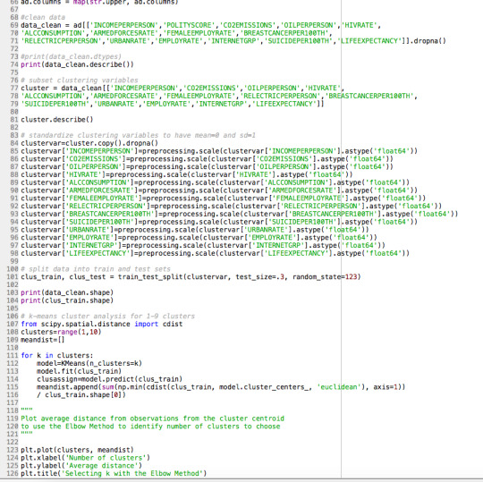
Code:
Results/Interpretation
INCOMEPERPERSON POLITYSCORE CO2EMISSIONS OILPERPERSON HIVRATE \
count 55.00 55.00 55.00 55.00 55.00
mean 12627.14 6.29 17031173042.43 1.08 0.58
std 12545.77 5.89 47219858116.11 0.85 2.38
min 558.06 -10.00 226255333.30 0.03 0.06
25% 2515.64 5.50 1914313500.00 0.44 0.10
50% 6105.28 9.00 4200940333.00 0.81 0.20
75% 25278.09 10.00 11896311167.00 1.56 0.40
max 39972.35 10.00 334000000000.00 4.21 17.80
ALCCONSUMPTION ARMEDFORCESRATE FEMALEEMPLOYRATE \
count 55.00 55.00 55.00
mean 9.57 1.17 46.97
std 5.20 0.82 10.86
min 0.05 0.29 18.20
25% 6.56 0.53 41.90
50% 10.08 0.96 48.00
75% 13.17 1.58 54.45
max 19.15 3.71 68.90
BREASTCANCERPER100TH RELECTRICPERPERSON URBANRATE EMPLOYRATE \
count 55.00 55.00 55.00 55.00
mean 50.26 1461.08 67.49 57.40
std 25.22 1483.93 16.14 7.60
min 16.60 68.12 27.14 41.10
25% 30.55 491.13 60.87 51.85
50% 46.00 830.70 68.46 57.90
75% 74.60 1909.12 77.42 61.90
max 101.10 7432.13 95.64 76.00
INTERNETGRP SUICIDEPER100TH LIFEEXPECTANCY
count 55.00 55.00 55.00
mean 0.49 11.11 75.40
std 0.50 7.04 5.79
min 0.00 1.38 52.80
25% 0.00 5.95 73.05
50% 0.00 10.06 75.63
75% 1.00 13.86 80.49
max 1.00 33.34 83.39
(55, 15)
(38, 14)
/Users/user/anaconda/lib/python3.5/site-packages/sklearn/preprocessing/data.py:167: UserWarning: Numerical issues were encountered when centering the data and might not be solved. Dataset may contain too large values. You may need to prescale your features.
warnings.warn(“Numerical issues were encountered ”
Cluster frequency
0 23
1 15
Name: cluster, dtype: int64
Clustering variable means by cluster
index INCOMEPERPERSON CO2EMISSIONS OILPERPERSON HIVRATE \
cluster
0 81.39 -0.64 -0.21 -0.47 0.18
1 85.07 1.34 0.37 1.18 -0.16
ALCCONSUMPTION ARMEDFORCESRATE FEMALEEMPLOYRATE \
cluster
0 -0.01 �� 0.35 -0.32
1 0.19 -0.60 0.64
RELECTRICPERPERSON BREASTCANCERPER100TH SUICIDEPER100TH URBANRATE \
cluster
0 -0.57 -0.54 0.10 -0.31
1 1.23 1.22 -0.16 0.75
EMPLOYRATE INTERNETGRP LIFEEXPECTANCY
cluster
0 -0.26 -0.55 -0.62
1 0.61 1.02 0.88
OLS Regression Results
=======================================================================Dep. Variable: POLITYSCORE R-squared: 0.115
Model: OLS Adj. R-squared: 0.090
Method: Least Squares F-statistic: 4.678
Date: Mon, 12 Dec 2016 Prob (F-statistic): 0.0373
Time: 13:37:24 Log-Likelihood: -122.22
No. Observations: 38 AIC: 248.4
Df Residuals: 36 BIC: 251.7
Df Model: 1
Covariance Type: nonrobust
========================================================================
coef std err t P>|t| [95.0% Conf. Int.]
———————————————————————————–
Intercept 4.2174 1.293 3.263 0.002 1.596 6.839
C(cluster)[T.1] 4.4493 2.057 2.163 0.037 0.277 8.622
=======================================================================
Omnibus: 16.374 Durbin-Watson: 1.597
Prob(Omnibus): 0.000 Jarque-Bera (JB): 18.322
Skew: -1.554 Prob(JB): 0.000105
Kurtosis: 4.383 Cond. No. 2.44
=======================================================================
Warnings:
[1] Standard Errors assume that the covariance matrix of the errors is correctly specified.
means for POLITYSCORE by cluster
POLITYSCORE
cluster
0 4.22
1 8.67
standard deviations for POLITYSCORE by cluster
POLITYSCORE
cluster
0 6.78
1 5.16
Multiple Comparison of Means - Tukey HSD,FWER=0.05
==========================================
group1 group2 meandiff lower upper reject
——————————————
0 1 4.4493 0.277 8.6215 True
——————————————
Figure 1. Elbow curve of r-square values for the nine cluster solutions
Summaries
The elbow curve was inconclusive, suggesting that the 2 and 6-cluster solutions might be interpreted. The results below are for an interpretation of the 2-cluster solution.
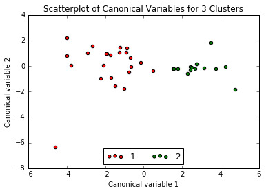
Canonical discriminant analyses was used to reduce the 14 clustering variable down a few variables that accounted for most of the variance in the clustering variables. A scatterplot of the first two canonical variables by cluster (Figure 2 shown below) indicated that the observations in clusters 1 and 2 were sparely packed with relatively low within cluster variance, and did not overlap each other. Observations in cluster 1 were spread out more than clusters 2, showing high within cluster variance. The results of this plot suggest that the best cluster solution may have fewer than 3 clusters, so it will be especially important to also evaluate the cluster solutions with fewer than 3 clusters.
Figure 2. Plot of the first two canonical variables for the clustering variables by cluster.
Pattern of Means
The means on the clustering variables showed that, compared to the other clusters, countries in cluster 1 had highest levels on the clustering variables. They had a relatively low likelihood of HIV, armed forces and suicide rates. Countries in cluster 0 had low income levels, oil use rate, co2 emissions, alcohol consumption, female employment rate, residential electricity, breast cancer, urbanization rate, employment rate, low internet use rate and life expectancy rate, and high HIV rate and armed forces. The R square and F statistic value from above show that the clusters differ non-significantly on Polity score.
ANOVA - How the clusters differ on Polity Score
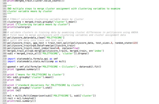
In order to externally validate the clusters, an Analysis of Variance (ANOVA) was conducting to test for significant differences between the clusters on polity score (democracy level). A tukey test was used for post hoc comparisons between the clusters. Results indicated significant differences between the clusters on Polity score with p<.05 and F-statistics of 4.68
Countries in cluster 1 have the largest per person polity score (mean = 8.67, s.d = 5.16) while countries in cluster 0 have the lowest polity score globally (mean = 4.22, s.d = 6.78).
0 notes
Text
LassoRegression
The Gapminder data set have been consistently used in all my models and assignments.
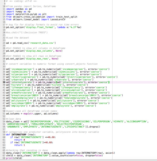
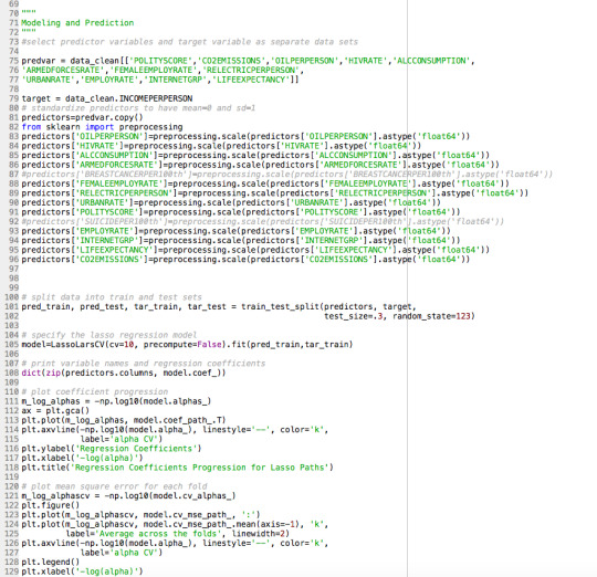
A lasso regression analysis was conducted to identify a subset of variables from a pool of 12 categorical and quantitative predictor variables that best predicted a quantitative response variable measuring income levels of countries. Categorical predictor included internet use rate a series of 1 binary categorical variable (internetgrp) for low and high internet use rate to improve interpretability of the selected model with fewer predictors. Quantitative predictor variables include, co2 emissions, oil per person, electricity use per person, internet use rate, HIV rate, life expectancy, alcohol consumption rate, female employment rate, armed forces rate, political scores, urbanization rate and employment rate. An attempt was made to standardized all predictor variable to have a mean of zero and a standard deviation of one.
Data were randomly split into a training set that included 70% of the observations (N=39) and a test set that included 30% of the observations (N=16). The least angle regression algorithm with k=10 fold cross validation was used to estimate the lasso regression model in the training set, and the model was validated using the test set. The change in the cross validation average (mean) squared error at each step was used to identify the best subset of predictor variables.
Results and Interpretation
Results
0 28
1 27
Name: INTERNETGRP, dtype: int64
{‘POLITYSCORE’: 0.0,
'FEMALEEMPLOYRATE’: 0.0,
'CO2EMISSIONS’: 1068.7187529092107,
'ARMEDFORCESRATE’: -723.2926183357024,
'EMPLOYRATE’: 776.54122203172199,
'INTERNETGRP’: 2367.5929322737056,
'ALCCONSUMPTION’: 0.0,
'OILPERPERSON’: 1270.8850125927634,
'RELECTRICPERPERSON’: 4152.4352947049692,
'HIVRATE’: 1933.4732242605226,
'URBANRATE’: -119.50922579487808,
'LIFEEXPECTANCY’: 4788.3810162737091}
/Users/user/anaconda/lib/python3.5/site-packages/sklearn/preprocessing/data.py:167: UserWarning: Numerical issues were encountered when centering the data and might not be solved. Dataset may contain too large values. You may need to prescale your features.
warnings.warn(“Numerical issues were encountered ”
training data MSE
20362652.1359
test data MSE
28666821.5623
training data R-square
0.879819425788
test data R-square
0.712225617637
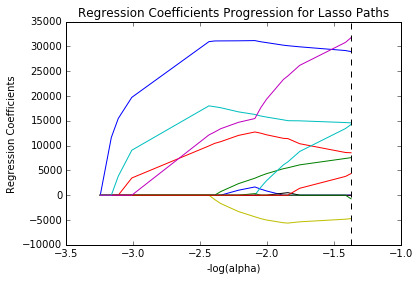
Figure 1 above shows the relative importance of the predictors and the steps in which each variable enters the model. The standardization of the predictors to have a mean of 1 and standard deviation of 0 did not work because of the large variability in the predictor values. However, based on the regression coefficients stated above, Life Expectancy rate represented by the blue line had the largest regression coefficient and was therefore entered into the model first, followed by electricity use rate, the sea blue line at step 2 and internet grp rate, the red line at step 3 and so on.
Interpretation
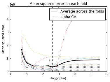
Figure 2 above shows the change in the validation mean square error at each step. Initially it decreases rapidly and gets to a plateau or levels off at which point adding more predictors doesn’t lead to much reduction in the mean square error. The behaviour is expected as model complexity increases.
The test MSE (28666821.5623) was closed to the training MSE (20362652.1359) suggesting the prediction accuracy was pretty stable across the 2 datasets.
The R-square of 0.88 and 0.71 indicating the selected model predictors predicts 88% and 71% of the variability in income levels in training and test datasets, respectively.
Conclusion
Of the 12 predictor variables, 9 were retained in the selected model. During the estimation process, life expectancy rate and electricity use rate were the most strongly associated with income level response variable, followed by internet group rate. Armed forces rate and urban rate were negatively associated with income level and the rest of the 7 predictors (co2 emissions, oil per person, electricity use per person, internet use rate, HIV rate, life expectancy and employment rate) were positively associated with income level. These 9 variables accounted for 71% of the variance in the income level response variable
0 notes
Text
Dataset
Similar to the Decision Trees assignment 1, my data set came from Gapminder for the purpose of running Random Forest analysis.
Data Management
I binned my target variable, internetgrp (internetuserate) in zero (countries with less internet use rate) and (1: countries with high internet use rate.
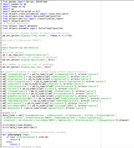
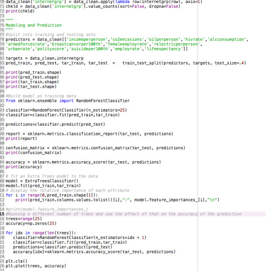
Code
Output and Interpretation
type: object
incomeperperson co2emissions oilperperson hivrate alcconsumption \
count 55.00 55.00 55.00 55.00 55.00
mean 12627.14 17031173042.43 1.08 0.58 9.57
std 12545.77 47219858116.11 0.85 2.38 5.20
min 558.06 226255333.30 0.03 0.06 0.05
25% 2515.64 1 914313500.00 0.44 0.10 6.56
50% 6105.28 4200940333.00 0.81 0.20 10.08
75% 25278.09 11896311167.00 1.56 0.40 13.17
max 39972.35 334000000000.00 4.21 17.80 19.15
armedforcesrate breastcancerper100th femaleemployrate \
count 55.00 55.00 55.00
mean 1.17 50.26 46.97
std 0.82 25.22 10.86
min 0.29 16.60 18.20
25% 0.53 30.55 41.90
50% 0.96 46.00 48.00
75% 1.58 74.60 54.45
max 3.71 101.10 68.90
relectricperperson urbanrate polityscore suicideper100th \
count 55.00 55.00 55.00 55.00
mean 1461.08 67.49 6.29 11.11
std 1 483.93 16.14 5.89 7.04
min 68.12 27.14 -10.00 1.38
25% 491.13 60.87 5.50 5.95
50% 830.70 68.46 9.00 10.06
75% 1909.12 77.42 10.00 13.86
max 7432.13 95.64 10.00 33.34
employrate internetuserate lifeexpectancy
count 55.00 55.00 55.00
mean 57.40 52.12 75.40
std 7.60 26.34 5.79
min 41.10 3.70 52.80
25% 51.85 32.72 73.05
50% 57.90 46.68 75.63
75% 61.90 77.57 80.49
max 76.00 93.28 83.39
0 28
1 27
Name: internetgrp, dtype: int64
(33, 14)
(22, 14)
(33,)
(22,)
Summary Classification report
precision recall f1-score support
0 0.89 1.00 0.94 8
1 1.00 0.93 0.96 14
avg / total 0.96 0.95 0.96 22
Shape
(33, 14)
(22, 14)
(33,)
(22,)
The shape above indicates the shape of the training and test samples. There are 33 observations with 60% of the dataset used as training set and 40% observations are used as test set. There is one target variable, internetgrp and 14 predictor variables used in this model.
Predictions
[ 8 0]
[ 1 13]]
The matrix above indicates the output of confusion matrix. The diagonal, 8, 13 indicates the number of true negatives and true positives respectively, for the internet use rate. The diagonal 0, 1 indicates the false negatives and false positives. Internetgrp 0 represents countries with low internet rates and internetgrp 1 indicate countries with high internet use rate.
The accuracy of the model came up as 0.954545454545. This means almost 95% of the sample of countries was classified correctly as having a low or high internet use rate.
Features Relative Importance
incomeperperson : 0.282991943842
co2emissions : 0.0118818681319
oilperperson : 0.156751663465
hivrate : 0.0321745852187
alcconsumption : 0.0927978761732
armedforcesrate : 0.0417505494505
breastcancerper100th : 0.129482079891
femaleemployrate : 0.0112820512821
relectricperperson : 0.0607948717949
urbanrate : 0.0161730769231
polityscore : 0.0216474358974
suicideper100th : 0.0216978021978
employrate : 0.0370192307692
lifeexpectancy : 0.0835549649626
Conclusions
Random forest analysis was performed to evaluate the importance of a series of predictors (quantitative explanatory variables) to predict a binary, target (categorical response) variable.
The above table of explanatory variable were used as model predictors. The variable with the highest and lowest important votes were incomeperperson (
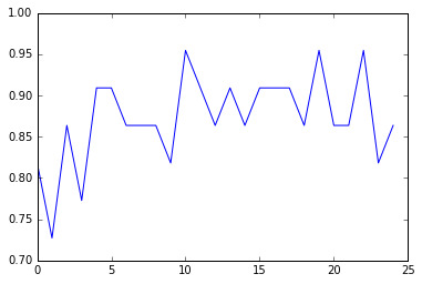
0.282991943842) and femaleemployrate ( 0.0112820512821), respectively. Including more predictor variables improved the model from 85% to 95%.
0 notes
Text
My data set is Gapminder dataset. The Decision tree analysis is to test nonlinear relationships among a series of explanatory variables and a binary, categorical response variable.
Data Preparation
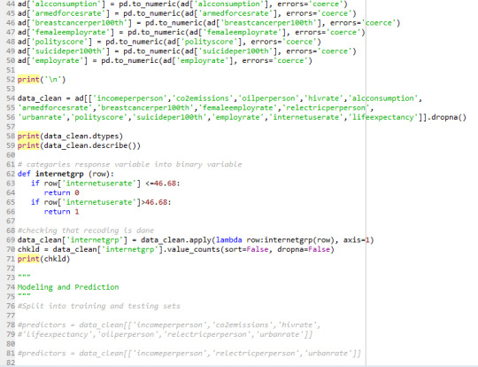
The Gapminder dataset does not have any binary categorical variable. So, I did convert ‘internetuserate’ into a binary categorical variable. The variable internetgrp ranges from 3.7 to 93.28; internetgrp <= 46.68 is deemed low internet usage and >46.68 is considered high internet usage. The categorizes countries in low and high internet usage countries.
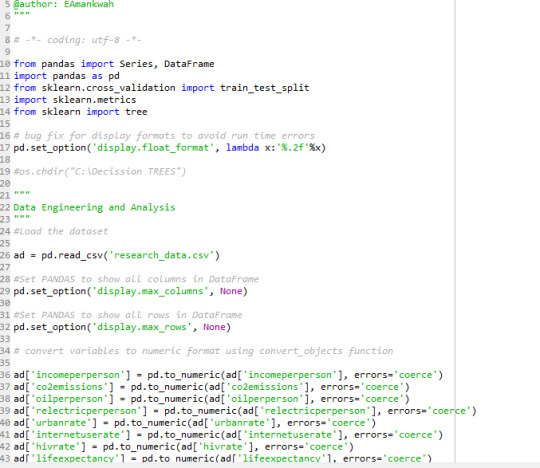
Code
Output
incomeperperson co2emissions oilperperson hivrate alcconsumption \
count 55.00 55.00 55.00 55.00 55.00
mean 12627.14 17031173042.43 1.08 0.58 9.57
std 12545.77 47219858116.11 0.85 2.38 5.20
min 558.06 226255333.30 0.03 0.06 0.05
25% 2515.64 1914313500.00 0.44 0.10 6.56
50% 6105.28 4200940333.00 0.81 0.20 10.08
75% 25278.09 11896311167.00 1.56 0.40 13.17
max 39972.35 334000000000.00 4.21 17.80 19.15
armedforcesrate breastcancerper100th femaleemployrate \
count 55.00 55.00 55.00
mean 1.17 50.26 46.97
std 0.82 25.22 10.86
min 0.29 16.60 18.20
25% 0.53 30.55 41.90
50% 0.96 46.00 48.00
75% 1.58 74.60 54.45
max 3.71 101.10 68.90
relectricperperson urbanrate polityscore suicideper100th \
count 55.00 55.00 55.00 55.00
mean 1461.08 67.49 6.29 11.11
std 1483.93 16.14 5.89 7.04
min 68.12 27.14 -10.00 1.38
25% 491.13 60.87 5.50 5.95
50% 830.70 68.46 9.00 10.06
75% 1909.12 77.42 10.00 13.86
max 7432.13 95.64 10.00 33.34
employrate internetuserate lifeexpectancy
count 55.00 55.00 55.00
mean 57.40 52.12 75.40
std 7.60 26.34 5.79
min 41.10 3.70 52.80
25% 51.85 32.72 73.05
50% 57.90 46.68 75.63
75% 61.90 77.57 80.49
max 76.00 93.28 83.39
0 28
1 27
Name: internetgrp, dtype: int64
(33, 2)
(22, 2)
(33,)
(22,)
[[12 2]
[2 6]]
0.818181818182
Tree
Interpretations
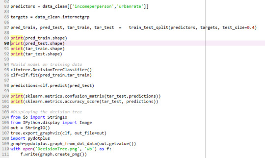
The output shows the shape of the training and test samples. 33 observations, 60% of the dataset is used as training set and the remaining 40% observations are used as test set. There are seven predictors (incomeperperson, co2emissions, hivrate, lifeexpectancy, oilperperson, relectricperperson and urbanrate;explanatory variables) used in this analysis and one target (internetuserate; response) variable. The results were inconsistent and hence, I reduced the predictor variable to 2 (incomperperson and urbanrate) inorder to get a fell of the decision tree output.
[[12 2]
[ 2 6]]
The diagonal, 12, 6 indicates the number of true negatives and true positives respectively. The diagonal 2, 2 reflects the false negatives and false positives for the variable internetgrp. The value of 1 for the target means the country has high internet use rate and 0 constitute low internet use.
The accuracy of the model is 0.818181818182
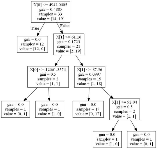
The picture above shows the classified tree generated based on the Gini Index. The Gini index creates binary slits using the formula sum of probability for success or failure. The two variables x[0] and x[1] make up the tree, predictor variables.
The tree began at incomeperperson<=4942.0605 and grew till Gini index became zero in all the branches. The second predictor used in the classification was urbanrate.
The tree began with 33 training samples and categorized the different samples into low and high internet use rate countries.
Tree interpretation/Summary
The first split of the tree shows if incomeperperson; x [0] <=4942.0605 is true (first slip to the left), which means countries with income levels less than 4942.1 represented by 12 samples out of the 33 training samples, all the 12 samples are classified as low internet use rate countries and 0 (0%) high internet use rate countries. If incomeperperson, x [0] <=4942.0605 is false and urbanrate <=61.16 is true (first slit to the right), the tree branches left and represented I sample (50%) with low internet use rate and 1 sample (50%) high internet use rate when incomperperson is <=12661.34. The last node on the far right indicated if urbanrate<=92.04 is true, 1 sample (1 country; 100%) has low internet use rate. However, if urbanrate<=92.04 is false, 1 sample (1 countre,100%) has high internet use rate.
0 notes
Text
My Research:
My research question was to establish the relationship and possible causality between economic growth (income levels), global pollution (co2 emissions levels), oil use rate in Canada and Ghana but was executed to include all the 192 NU countries and other areas. The relationship was later extended to include electricity use and internet use rate among these countries.
Sample and measure
The aim of this assignment is to analysis the association and model fit among the following variables from the Gapminder dataset.
Explanatory variables – Incomeperperson, urbanrate, relectricperperson, co2 emissions
Response - variable oiluserate
*Caution: The coding and output in this assignment are long because all the tools and test taught in this section of the course were exploited.
Code
import numpy as np
import pandas as pd
import statsmodels.api as sm
import statsmodels.formula.api as smf
import seaborn as sb
import matplotlib.pyplot as plt
# bug fix for display formats to avoid run time errors
pd.set_option(‘display.float_format’, lambda x:’%.2f’%x)
#call in data set
ad = pd.read_csv('research_data.csv’)
#Set PANDAS to show all columns in DataFrame
pd.set_option('display.max_columns’, None)
#Set PANDAS to show all rows in DataFrame
pd.set_option('display.max_rows’, None)
# convert variables to numeric format using convert_objects function
ad['incomeperperson’] = pd.to_numeric(ad['incomeperperson’], errors='coerce’)
ad['co2emissions’] = pd.to_numeric(ad['co2emissions’], errors='coerce’)
ad['oilperperson’] = pd.to_numeric(ad['oilperperson’], errors='coerce’)
ad['relectricperperson’] = pd.to_numeric(ad['relectricperperson’], errors='coerce’)
ad['urbanrate’] = pd.to_numeric(ad['urbanrate’], errors='coerce’)
ad['internetuserate’] = pd.to_numeric(ad['internetuserate’], errors='coerce’)
print(’\n’)
#clean data
data_clean = ad[['incomeperperson’, 'co2emissions’ , 'oilperperson’ , 'relectricperperson’ , 'urbanrate’ , 'internetuserate’]].dropna()
# POLYNOMIAL REGRESSION
# first order (linear) scatterplot
scat1 = sb.regplot(x=“incomeperperson”, y=“oilperperson”, scatter=True, data=data_clean)
plt.xlabel('Income Levels’)
plt.ylabel('Oil Use Rate’)
plt.show()
# fit second order polynomial
# run the 2 scatterplots together to get both linear and second order fit lines
scat1 = sb.regplot(x=“incomeperperson”, y=“oilperperson”, scatter=True, order=2, data=data_clean)
plt.xlabel('Income Levels’)
plt.ylabel('Oil Use Rate’)
plt.show()
# center quantitative IVs for regression analysis
data_clean['incomeperperson_c’] = (data_clean['incomeperperson’] - data_clean['incomeperperson’].mean())
print(’\n’)
print(data_clean['incomeperperson_c’].mean())
data_clean['co2emissions_c’] = (data_clean['co2emissions’] - data_clean['co2emissions’].mean())
print(’\n’)
print(data_clean['co2emissions_c’].mean())
data_clean['urbanrate_c’] = (data_clean['urbanrate’] - data_clean['urbanrate’].mean())
print(’\n’)
print(data_clean['urbanrate_c’].mean())
data_clean[[“incomeperperson_c”, “co2emissions_c”]].describe()
# Testing relationship of electricity use rate and urban use rate with oil use rate
reg1=smf.ols('oilperperson ~ relectricperperson + urbanrate_c’,data=data_clean).fit()
print (reg1.summary())
print(’\n’)
# Testing income levels as another explanatory variable
reg2=smf.ols('oilperperson ~ incomeperperson’,data=data_clean).fit()
print (reg2.summary())
print(’\n’)
# Testing income levels as a potential confounder while controlling electric use rate
reg3=smf.ols('oilperperson ~ incomeperperson + relectricperperson’,data=data_clean).fit()
print (reg3.summary())
print(’\n’)
# adding more variables to evaluate multiple predictors among several independent variables
reg4=smf.ols('oilperperson ~ relectricperperson + incomeperperson + co2emissions_c + urbanrate_c + internetuserate’,
data=data_clean).fit()
print (reg4.summary())
print(’\n’)
# linear regression analysis
reg5 = smf.ols('oilperperson ~ incomeperperson_c’, data=data_clean).fit()
print(’\n’)
print (reg5.summary())
print(’\n’)
# quadratic (polynomial) regression analysis
# run following line of code if you get PatsyError 'ImaginaryUnit’ object is not callable
#del I
reg6 = smf.ols('oilperperson ~ incomeperperson_c + I(incomeperperson_c**2)’, data=data_clean).fit()
print(’\n’)
print (reg6.summary())
print(’\n’)
# EVALUATING MODEL FIT
# adding co2 emissions pollution
reg7 = smf.ols('oilperperson ~ incomeperperson_c + I(incomeperperson_c**2) + co2emissions_c’, data=data_clean).fit()
print (reg7.summary())
print(’\n’)
#Q-Q plot for normality
fig1=sm.qqplot(reg7.resid, line='r’)
plt.ylabel(“Theoretical quantitiles”,size=24)
plt.xlabel(“Experimental quantiles”, size=24)
plt.show()
print(’\n’)
# simple plot of residuals
stdres=pd.DataFrame(reg7.resid_pearson)
fig2=plt.plot(stdres, 'o’, ls='None’)
I = plt.axhline(y=0, color='r’)
plt.ylabel('Standardized Residual’)
plt.xlabel('Observation Number’)
print(’\n’)
print(fig2)
# additional regression diagnostic plots
fig3 = plt.figure() #(figsize(12,8))
fig3 = sm.graphics.plot_regress_exog(reg7, “co2emissions_c”, fig=fig3)
# leverage plot
fig4=sm.graphics.influence_plot(reg7, size=8)
print(’\n’)
print(fig4)
OUTPUT/RESULTS
Centering variables
Variable
Incomperperson_c
Co2emission_c
Urbanrate_c
Mean
incomeperperson_c - 1.48e-12
c02emissions_c - -6.47e-08
urbanrate_c - -4.82-16
Since all the mean values were close to zero, all the variables were properly centered
Results 1: Testing relationship of electric use rate and urban use rate with oil use rate
LS Regression Results
==============================================================================
Dep. Variable: oilperperson R-squared: 0.673
Model: OLS Adj. R-squared: 0.661
Method: Least Squares F-statistic: 57.51
Date: Tue, 22 Nov 2016 Prob (F-statistic): 2.66e-14
Time: 15:52:03 Log-Likelihood: -51.475
No. Observations: 59 AIC: 109.0
Df Residuals: 56 BIC: 115.2
Df Model: 2
Covariance Type: nonrobust
======================================================================================
coef std err t P>|t| [95.0% Conf. Int.]
————————————————————————————–
Intercept 0.6029 0.106 5.693 0.000 0.391 0.815
relectricperperson 0.0004 4.43e-05 8.188 0.000 0.000 0.000
urbanrate_c 0.0154 0.005 2.936 0.005 0.005 0.026
==============================================================================
Omnibus: 35.884 Durbin-Watson: 2.005
Prob(Omnibus): 0.000 Jarque-Bera (JB): 102.828
Skew: 1.765 Prob(JB): 4.69e-23
Kurtosis: 8.420 Cond. No. 3.45e+03
==============================================================================
Warnings:
[1] Standard Errors assume that the covariance matrix of the errors is correctly specified.
[2] The condition number is large, 3.45e+03. This might indicate that there are
strong multicollinearity or other numerical problems.
Summary 1
Both electric use rate and urban rate (explanatory variables) had Pvalues less than 0.05 indicating they were positively associated with the oil use rate (response variable). They are positively related to the oil use rate since their coefficients are positive. The linear relationship has a R-square value of 0.0673 indicated about 67.3 % level of variability in the oil use rate that can be explained by both electric use rate and urban use rate.
Results 2: Testing income levels (incomeperperson) as another explanatory variable
OLS Regression Results
==============================================================================
Dep. Variable: oilperperson R-squared: 0.432
Model: OLS Adj. R-squared: 0.422
Method: Least Squares F-statistic: 43.31
Date: Tue, 22 Nov 2016 Prob (F-statistic): 1.58e-08
Time: 15:52:03 Log-Likelihood: -67.736
No. Observations: 59 AIC: 139.5
Df Residuals: 57 BIC: 143.6
Df Model: 1
Covariance Type: nonrobust
===================================================================================
coef std err t P>|t| [95.0% Conf. Int.]
———————————————————————————–
Intercept 0.5169 0.144 3.582 0.001 0.228 0.806
incomeperperson 5.462e-05 8.3e-06 6.581 0.000 3.8e-05 7.12e-05
==============================================================================
Omnibus: 52.395 Durbin-Watson: 2.123
Prob(Omnibus): 0.000 Jarque-Bera (JB): 229.421
Skew: 2.548 Prob(JB): 1.52e-50
Kurtosis: 11.207 Cond. No. 2.48e+04
==============================================================================
Warnings:
[1] Standard Errors assume that the covariance matrix of the errors is correctly specified.
[2] The condition number is large, 2.48e+04. This might indicate that there are
strong multicollinearity or other numerical problems.
Summary 2
P=000 is significant, coeff=5.5e-5 and R-square = 0.432 means income per person is positively associated and amount of variability in the oil use rate causes (43%) can be explained by income levels. Based on the sampled parameter estimate, it is 95% assured that the population parameter will fall somewhere between the lower and upper limits of 0.23 and 0.81. Beta 1 estimate value of income level indicate positive change or 5.7e-05 per one unit of change, indicating slight positive slope of regression model line. The governing equation is oilperperson = 0.5 + 5.5e-05*incomeperperson
Results 3: Testing income levels (incomeperperson) as a potential confounder while controlling electric use rate
OLS Regression Results
==============================================================================
Dep. Variable: oilperperson R-squared: 0.652
Model: OLS Adj. R-squared: 0.639
Method: Least Squares F-statistic: 52.40
Date: Tue, 22 Nov 2016 Prob (F-statistic): 1.49e-13
Time: 15:52:03 Log-Likelihood: -53.294
No. Observations: 59 AIC: 112.6
Df Residuals: 56 BIC: 118.8
Df Model: 2
Covariance Type: nonrobust
======================================================================================
coef std err t P>|t| [95.0% Conf. Int.]
———————————————————————���————–
Intercept 0.4101 0.115 3.554 0.001 0.179 0.641
incomeperperson 1.93e-05 8.85e-06 2.182 0.033 1.58e-06 3.7e-05
relectricperperson 0.0003 5.62e-05 5.947 0.000 0.000 0.000
==============================================================================
Omnibus: 46.531 Durbin-Watson: 1.875
Prob(Omnibus): 0.000 Jarque-Bera (JB): 207.027
Skew: 2.147 Prob(JB): 1.11e-45
Kurtosis: 11.110 Cond. No. 2.53e+04
==============================================================================
Warnings:
[1] Standard Errors assume that the covariance matrix of the errors is correctly specified.
[2] The condition number is large, 2.53e+04. This might indicate that there are
strong multicollinearity or other numerical problems.
Summary 3
The explanatory variables, income levels and electric use rate have been found to be separately significant and associate with the oil use rate. When both variables are included in the model and the income level is controlled, the two variables are still significantly associated with the oil use rate. This indicates that the income level variable is not a potential confounder. However, the estimated R-square increased from 0.432 to 0.652, indicating that the amount of variability in the oil use rate that can be explained by the combined effect of both income levels and electric use rate has increased from 43% to 65%.
Results 4: Testing the effect of adding more explanatory variables to evaluate multiple predictors among several independent variables
OLS Regression Results
==============================================================================
Dep. Variable: oilperperson R-squared: 0.686
Model: OLS Adj. R-squared: 0.656
Method: Least Squares F-statistic: 23.12
Date: Tue, 22 Nov 2016 Prob (F-statistic): 3.07e-12
Time: 15:52:03 Log-Likelihood: -50.269
No. Observations: 59 AIC: 112.5
Df Residuals: 53 BIC: 125.0
Df Model: 5
Covariance Type: nonrobust
======================================================================================
coef std err t P>|t| [95.0% Conf. Int.]
————————————————————————————–
Intercept 0.6395 0.219 2.914 0.005 0.199 1.080
relectricperperson 0.0003 5.56e-05 5.810 0.000 0.000 0.000
incomeperperson 1.761e-05 1.29e-05 1.368 0.177 -8.21e-06 4.34e-05
co2emissions_c -5.824e-14 1.85e-12 -0.032 0.975 -3.76e-12 3.64e-12
urbanrate_c 0.0144 0.006 2.379 0.021 0.002 0.026
internetuserate -0.0037 0.006 -0.642 0.523 -0.015 0.008
==============================================================================
Omnibus: 40.861 Durbin-Watson: 1.922
Prob(Omnibus): 0.000 Jarque-Bera (JB): 152.938
Skew: 1.902 Prob(JB): 6.17e-34
Kurtosis: 9.910 Cond. No. 1.28e+11
==============================================================================
Warnings:
[1] Standard Errors assume that the covariance matrix of the errors is correctly specified.
[2] The condition number is large, 1.28e+11. This might indicate that there are
strong multicollinearity or other numerical problems.
Summary 4
The analysis above show that three explanatory variables (income levels, co2 emissions and internet use rate) with p values greater than 0.05 and confidence intervals including zeros, were not associated with the oil use rate. However, the level of variability in the oil use rate that can be explained by multiple (several) explanatory variables is higher (R-squared =0.686) than when one explanatory variable (R-squared =0.432) or two explanatory variables (R-squared =0.625) were included in the model. This shows that model results can be improved when more explanatory variables are included in the model. The Pvalue of incomeperperson is 0.177>0.05, indicating the null hypothesis that there is no association between income levels and oil use cannot be rejected. The income level variable appears to behave as a confounder in this scenario (Pvalue was significant in the previous scenarios (p=0.033).
Results5: Testing zero order polynomial regression analysis
OLS Regression Results
==============================================================================
Dep. Variable: oilperperson R-squared: 0.432
Model: OLS Adj. R-squared: 0.422
Method: Least Squares F-statistic: 43.31
Date: Tue, 22 Nov 2016 Prob (F-statistic): 1.58e-08
Time: 15:52:03 Log-Likelihood: -67.736
No. Observations: 59 AIC: 139.5
Df Residuals: 57 BIC: 143.6
Df Model: 1
Covariance Type: nonrobust
=====================================================================================
coef std err t P>|t| [95.0% Conf. Int.]
————————————————————————————-
Intercept 1.1951 0.101 11.830 0.000 0.993 1.397
incomeperperson_c 5.462e-05 8.3e-06 6.581 0.000 3.8e-05 7.12e-05
==============================================================================
Omnibus: 52.395 Durbin-Watson: 2.123
Prob(Omnibus): 0.000 Jarque-Bera (JB): 229.421
Skew: 2.548 Prob(JB): 1.52e-50
Kurtosis: 11.207 Cond. No. 1.22e+04
==============================================================================
Warnings:
[1] Standard Errors assume that the covariance matrix of the errors is correctly specified.
[2] The condition number is large, 1.22e+04. This might indicate that there are
strong multicollinearity or other numerical problems.
Summary 5
P=000 is significant, coeff=5.4e-5 means income levels is positively and moderately associated with oil use rate. This also means that the absence of income levels is associated with a smaller number of oil use rate. R-square of the linear relationship = 0.432, indicating the amount of variability in oil use rate that can be explained by income level is 43%. Beta 1 estimate value of incomeperperson_c indicates positive change or 5.5e-05 per one unit of change, indicating slight positive slope of regression model line. The governing beta equation is oilperperson = 0.2 + 5.5e-05*incomeperperson_c.
Results 6: Testing quadratic (polynomial) analysis
OLS Regression Results
==============================================================================
Dep. Variable: oilperperson R-squared: 0.497
Model: OLS Adj. R-squared: 0.480
Method: Least Squares F-statistic: 27.72
Date: Tue, 22 Nov 2016 Prob (F-statistic): 4.29e-09
Time: 15:52:03 Log-Likelihood: -64.110
No. Observations: 59 AIC: 134.2
Df Residuals: 56 BIC: 140.5
Df Model: 2
Covariance Type: nonrobust
=============================================================================================
coef std err t P>|t| [95.0% Conf. Int.]
———————————————————————————————
Intercept 1.5336 0.158 9.733 0.000 1.218 1.849
incomeperperson_c 7.862e-05 1.19e-05 6.629 0.000 5.49e-05 0.000
I(incomeperperson_c ** 2) -2.285e-09 8.44e-10 -2.706 0.009 -3.98e-09 -5.94e-10
==============================================================================
Omnibus: 50.111 Durbin-Watson: 2.181
Prob(Omnibus): 0.000 Jarque-Bera (JB): 202.083
Skew: 2.453 Prob(JB): 1.31e-44
Kurtosis: 10.625 Cond. No. 3.72e+08
==============================================================================
Warnings:
[1] Standard Errors assume that the covariance matrix of the errors is correctly specified.
[2] The condition number is large, 3.72e+08. This might indicate that there are
strong multicollinearity or other numerical problems.
Summary 6
Figure 1
Figure 2
P values for both linear and second order are < 0.05 meaning both are significantly related to the oil use rate. A positive linear coefficient and a negative quadratic coefficient indicates the curve is concave such that it starts low then starts to go up and then go down again. R-square increased to 0.497 (from 43% to 50%) which means adding a quadratic term for income levels increases the amount of variability in oil use rate that can be explained by income levels. Hence the best fitting line for the association is the quadratic that includes some curvature. See figures 1 and 2 above. Beta estimate value of incomeperperson_c and incomeperperson_c**2 indicate positive and negative change, respectively, indicating a curvilinear (concave) shape. The governing beta equation is oilperperson = 1.5 + 7.9e-05*incomeperperson_c - 2.3e-9*incomeperperson_c**2
Results 7: Testing quadratic (polynomial) analysis while controlling a second explanatory variable
OLS Regression Results
==============================================================================
Dep. Variable: oilperperson R-squared: 0.498
Model: OLS Adj. R-squared: 0.471
Method: Least Squares F-statistic: 18.22
Date: Tue, 22 Nov 2016 Prob (F-statistic): 2.48e-08
Time: 15:52:03 Log-Likelihood: -64.056
No. Observations: 59 AIC: 136.1
Df Residuals: 55 BIC: 144.4
Df Model: 3
Covariance Type: nonrobust
=============================================================================================
coef std err t P>|t| [95.0% Conf. Int.]
———————————————————————————————
Intercept 1.5433 0.162 9.537 0.000 1.219 1.868
incomeperperson_c 7.847e-05 1.2e-05 6.558 0.000 5.45e-05 0.000
I(incomeperperson_c ** 2) -2.351e-09 8.76e-10 -2.682 0.010 -4.11e-09 -5.94e-10
co2emissions_c 7.286e-13 2.31e-12 0.315 0.754 -3.9e-12 5.36e-12
==============================================================================
Omnibus: 50.529 Durbin-Watson: 2.177
Prob(Omnibus): 0.000 Jarque-Bera (JB): 206.799
Skew: 2.470 Prob(JB): 1.24e-45
Kurtosis: 10.728 Cond. No. 7.59e+10
==============================================================================
Warnings:
[1] Standard Errors assume that the covariance matrix of the errors is correctly specified.
[2] The condition number is large, 7.59e+10. This might indicate that there are
strong multicollinearity or other numerical problems.
Summary 7:
The linear and quadratic Pvalues for income levels are still significant after adjusting for co2 emissions. Pvalue for co2 emissions is > 0.05 indicating co2 emissions are not significantly associated with oil use rate and that the null hypothesis cannot be neglected. The effect of the co2 emission rate is about 0.01% (49.8-49.7%). The governing beta equation is oilperperson = 1.5 + 7.9e-05*incomeperperson_c - 2.4e-9*incomeperperson_c**2 + 7.3e-13.
Results 8: Residual analysis
Figure 3
[<matplotlib.lines.Line2D object at 0x11886ac88>]
Figure(640x440)
Summary 8:
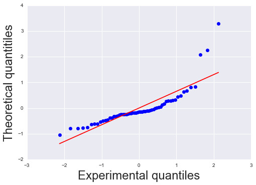
The qq plot above do not follow a straight line indicating the qq plot is not perfect normally distributed. The curvilinear curve may not be fully estimated by the quadratic term. This elicit for another explanatory variable to be included in the model which can improve the estimated observed curvilinearity.
Results 9: Standardized Residual analysis
Figure 4
Results 9: Standardized Residual analysis
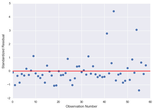
To estimate the overall fit of the observed values of the predicted response value and to look for outliers, I used standardized plot residuals, this is transformed to have a mean of 0 and standard deviation (Std) of 1. Most residuals fall within 1 Std of the mean (-1 to 1). A few have more than 2 Stds, above 2 or below -2. For a normal distribution, I expect that 95% of the values falls within 2 stds of the mean. About 3 values fall aside this range indicating the possibility of outliers. There is only 1 extreme outlier outside 3 Stds of the mean.
Results 10: contribution of specific explanatory values to the model fit
Figure 5
Summary 10
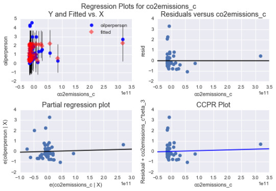
The above plots show how specific explanatory variables contribute to the fit of our model.
Top-right plot: the plot shows a week funnel shape pattern. The residual for each observation at different values of co2 emissions gets larger at lower co2 emissions and smaller when co2emissions increases. A second order co2emissions may be necessary in the model.
Lower left-the plot shows a partial residual regression typifying the effect of adding co2 emissions as an additional explanatory variable in the model giving that 1 or more explanatory variables are already in the model. The vertical axis shows residuals from the model of the other explanatory variable (income levels) excluding the co2 emissions. The horizontal axis is the residuals from the model of all the other explanatory variable in the model. The plot does not clearly indicate a non-linear relationship. The residuals are spread out around the partial regression line. Many of the values are far from the partial residual line indicating a great deal oil use rate prediction error. This confirms that the associated between and oil use rate is very weak after controlling income levels.
Results 11: leverage plot analysis
Figure 6
Summary 11: leverage plot analysis
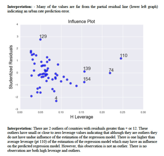
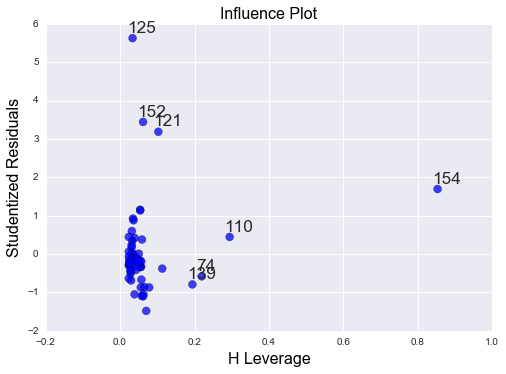
To examine observations that have an unusual large influence on the estimation of the predicted value of the response variable, oil use rate or outliers or both. There are 3 outliers of countries with residuals greater than +2. These outliers have small or close to zero leverage values indicating that although they are outliers they do not have undue influence of the estimation of the regression model. There is one higher than average leverage (pt 154) of the estimation of the regression model which may have an influence on the predicted regression model. However, this observation is not an outlier. There is no observation are both high leverage and outliers.
Conclusion
The hypothesis tested shows that there is association between some of the explanatory variables (income level, urban rate, internet use, electricity use) and the response variable (oil use rate). Th model fit better for quadratic polynomial than linear regression. As of now there is not enough evidence to prove causality.
0 notes
Text
Test A Basic Linear Reg.......
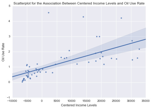
In this assignment, the relationship between income (explanatory variable) and oil use rate (response variable) is exploited. Linear regression coefficients between the income levels and oil use rate is determined. Also the income is centered such that the mean is very close to zero and the relationship between the centered income level and the oil use rate is exploited. Below is the code that I used:
mport numpy as np
import pandas as pd
import statsmodels.api
import statsmodels.formula.api as smf
import seaborn as sb
import matplotlib.pyplot as plt
# bug fix for display formats to avoid run time errors
pd.set_option(‘display.float_format’, lambda x:’%.2f’%x)
#call in data set
ad = pd.read_csv('research_data.csv’)
#Set PANDAS to show all columns in DataFrame
pd.set_option('display.max_columns’, None)
#Set PANDAS to show all rows in DataFrame
pd.set_option('display.max_rows’, None)
# convert variables to numeric format using convert_objects function
ad['incomeperperson’] = pd.to_numeric(ad['incomeperperson’], errors='coerce’)
ad['co2emissions’] = pd.to_numeric(ad['co2emissions’], errors='coerce’)
ad['oilperperson’] = pd.to_numeric(ad['oilperperson’], errors='coerce’)
#Centralize explanatory variable
ad[“incomeCentered”]= ad[“incomeperperson”] - np.mean(ad[“incomeperperson”])
np.mean(ad[“incomeCentered”])
#print('Checking the column types:\n’)
#print(ad.dtypes)
print(’\n’)
#clean data
data_clean = ad[['incomeperperson’, 'incomeCentered’,'co2emissions’ , 'oilperperson’ , 'relectricperperson’ , 'urbanrate’ , 'internetuserate’]].dropna()
#incomeperperson_mean=data_clean['incomeperperson’].mean()
sub1 = ad['incomeperperson’].mean()
print (sub1)
sub2 = ad['incomeCentered’].mean()
print (sub2)
# BASIC LINEAR REGRESSION
#Linear regression of Centered income level and oil use rate
scat1 = sb.regplot(x=“incomeCentered”, y=“oilperperson”, scatter=True, data=ad)
plt.xlabel('Centered Income Levels’)
plt.ylabel('Oil Use Rate’)
plt.title ('Scatterplot for the Association Between Centered Income Levels and Oil Use Rate’)
plt. show ()
print(’\n’)
print(scat1)
print(’\n’)
print (“OLS regression model for the association between centered income level and oil use rate”)
reg1 = smf.ols('incomeCentered ~ oilperperson’, data=data_clean).fit()
print (reg1.summary())
#Linear regression of income level and oil use rate
scat2 = sb.regplot(x=“incomeperperson”, y=“oilperperson”, scatter=True, data=ad)
plt.xlabel('Income Levels’)
plt.ylabel('Oil Use Rate’)
plt.title ('Scatterplot for the Association Between Income Levels and Oil Use Rate’)
plt. show ()
print(’\n’)
print(scat2)
print(’\n’)
print (“OLS regression model for the association between income level and oil use rate”)
reg2 = smf.ols('incomeperperson ~ oilperperson’, data=data_clean).fit()
print (reg2.summary())
Output
Mean of income Levels = 7164.842956180768
Mean of centred income levels = 1.125208188731892e-12
Comparing the mean, the mean of the centered value is so low it can be
considered to be 0, showing that our variable is centered.
The results of the scatter plot and the regression between the centered explanatory variable and the response variable:
Axes(0.125,0.125;0.775x0.775)
OLS regression model for the association between centered income level and oil use rate
OLS Regression Results
==============================================================================
Dep. Variable: incomeCentered R-squared: 0.432
Model: OLS Adj. R-squared: 0.422
Method: Least Squares F-statistic: 43.31
Date: Tue, 15 Nov 2016 Prob (F-statistic): 1.58e-08
Time: 21:01:49 Log-Likelihood: -622.05
No. Observations: 59 AIC: 1248.
Df Residuals: 57 BIC: 1252.
Df Model: 1
Covariance Type: nonrobust
================================================================================
coef std err t P>|t| [95.0% Conf. Int.]
——————————————————————————–
Intercept -4194.7052 1880.793 -2.230 0.030 -7960.929 -428.481
oilperperson 7904.4424 1201.091 6.581 0.000 5499.300 1.03e+04
==============================================================================
Omnibus: 6.758 Durbin-Watson: 1.684
Prob(Omnibus): 0.034 Jarque-Bera (JB): 7.852
Skew: 0.417 Prob(JB): 0.0197
Kurtosis: 4.581 Cond. No. 3.09
==============================================================================
The results of the scatter plot and the regression between the income level (non-centered) explanatory variable and the response variable:
Axes(0.125,0.125;0.775x0.775)
OLS regression model for the association between income level and oil use rate
OLS Regression Results
==============================================================================
Dep. Variable: incomeperperson R-squared: 0.432
Model: OLS Adj. R-squared: 0.422
Method: Least Squares F-statistic: 43.31
Date: Tue, 15 Nov 2016 Prob (F-statistic): 1.58e-08
Time: 21:01:49 Log-Likelihood: -622.05
No. Observations: 59 AIC: 1248.
Df Residuals: 57 BIC: 1252.
Df Model: 1
Covariance Type: nonrobust
================================================================================
coef std err t P>|t| [95.0% Conf. Int.]
——————————————————————————–
Intercept 2970.1378 1880.793 1.579 0.120 -796.086 6736.361
oilperperson 7904.4424 1201.091 6.581 0.000 5499.300 1.03e+04
==============================================================================
Omnibus: 6.758 Durbin-Watson: 1.684
Prob(Omnibus): 0.034 Jarque-Bera (JB): 7.852
Skew: 0.417 Prob(JB): 0.0197
Kurtosis: 4.581 Cond. No. 3.09
==============================================================================
In Summary, our linear regression has been proven successful, with a significant correlation with a p-value 1.58e-08 which is much lower than 0.05
The equation according to our results is:
oilperperson= 2970.1378 + 7904.4424 * incomperperson
oilperperson= -4194.7052 + 7904.4424 * incomeCentred
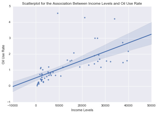
0 notes
Text
My Research:
My research question was to establish the relationship and possible causality between economic growth (income levels), global pollution (co2 emissions levels), oil use rate among Canada and Ghana but was executed to include all the 192 NU countries and other areas. The relationship was later extended to include electricity use and internet use rate among these countries.
Sample and measure
The sample of 5 indicators from GapMinder dataset (GapMnder), a non-profit foundation focusing on sustainable global development and achievement of the United Nations Millennium Development Goals. Currently, GapMinder has grown to include over 200 indicators, including gross domestic product, total employment rate, and estimated HIV prevalence, collected from reputable local, national and international organizations. The five indicators (samples) includes:
1) Income levels (incomeperperson; explanatory and moderator variable depending on the scenario ); measured in 2000 constant dollars in terms of gross domestic product per capita in 2000. The data comes from the World Band Work Development. The income level ranged from 103.78 to 105147.44, with a median of 2553.50
2) Pollution levels (co2emissions; response and explanatory variable depending on the scenario ); measured in metric tons in terms of total amount of co2 emissions between 1751 and 2006. The pollution level ranged from 132000 to 3.34e+11, with a median of 185901833.40.
3) Oil use rate (oilperperson; response variable); measured in tones per year per person in terms of consumption per capita in 2010.The data comes from British Petroleum, a global energy giant. The oil use rate ranged from 0.03 to 12.23, with a median of 1.03
4) Electricity use rate (relectricperperson; response variable); measured in kilo watt hour (kWh) in terms of residential electricity per person in 2008. The electricity use rate ranged from 0.00 to 11154.76, with a median of 597.14 and ;
5) Internet use rate (internetuserate; response variable ); measured in users per 10 people in terms of people with access to the world wide network. The internet use rate ranged from 10.21 to 95.64, with a median of 31.81
Data collection procedure
GapMinder dataset is collected from UN Statistics Division which ultimately come from economic statistics branch, international statistical agencies and national statistical services. Other sources include World Bank, Carbon Dioxide Information Analysis Centre (CDIC) and International Energy Agency. These datasets are made available for download through the GapMinder website (www.gapminder.org). At the local level, the data collection relies on researchers, professionals and private agencies operating in the individual countries.
For the current analysis, the income level is split into three categories, representing low income, medium income and high income groups.
0 notes
Text
Testing moderation and causation in the context of correlation: in the last assignment, I established that there is a positive and moderate Pearson correlation between electricity use and internet rate. This may mean that the more electricity an individual uses the more internet is used.
I found that there was a significant (P-value of 2.64e-7) association with correlation of 0.61. But the relationship between electricity use and internet use rate might differ based on countries with different income levels.
I explored this question by creating a third variable, income group variable, which is categorical. I categorized the new variable, the income-per-person which is quantitative, into high income countries, middle income countries, and low income countries. I created my income group variable which splits the sample of countries into low, middle, and high income groups using the dummy codes 1, 2, and 3. I then created three different data frames (sub1; low income countries, sub2; middle income countries and sub3; high income countries) that include only one income group each. Below is the code for the Pearson correlation, r and the P-value between the electricity use and internet use rate for each of the income groups.
# CORRELATION with Income groups as Moderator
import pandas as pd
import numpy as np
import scipy.stats
import seaborn as sb
import matplotlib.pyplot as plt
ad = pd.read_csv(‘research_data.csv’, low_memory=False)
#bug fix for display formats to avoid run time errors - put after code for loading data above
pd.set_option('display.float_format’, lambda x:’%f’%x)
#Set PANDAS to show all columns in DataFrame
pd.set_option('display.max_columns’, None)
#Set PANDAS to show all rows in DataFrame
pd.set_option('display.max_rows’, None)
# new code setting variables you will be working with to numeric
ad['incomeperperson’] = pd.to_numeric(ad['incomeperperson’], errors='coerce’)
ad['co2emissions’] = pd.to_numeric(ad['co2emissions’], errors='coerce’)
ad['oilperperson’] = pd.to_numeric(ad['oilperperson’], errors='coerce’)
ad['relectricperperson’] = pd.to_numeric(ad['relectricperperson’], errors='coerce’)
ad['urbanrate’] = pd.to_numeric(ad['urbanrate’], errors='coerce’)
ad['internetuserate’] = pd.to_numeric(ad['internetuserate’], errors='coerce’)
print('Checking the column types:\n’)
print(ad.dtypes)
print(’\n’)
data_clean = ad[['incomeperperson’, 'co2emissions’ , 'oilperperson’ , 'relectricperperson’ , 'urbanrate’ , 'internetuserate’]].dropna()
print (scipy.stats.pearsonr(data_clean['relectricperperson’], data_clean['internetuserate’]))
print(’\n’)
def incomegrp (row):
if row['incomeperperson’] <= 744.239:
return 1
elif row['incomeperperson’] <= 9425.326 :
return 2
elif row['incomeperperson’] > 9425.326:
return 3
data_clean['incomegrp’] = data_clean.apply (lambda row: incomegrp (row),axis=1)
chk1 = data_clean['incomegrp’].value_counts(sort=False, dropna=False)
print(chk1)
print(’\n’)
sub1=data_clean[(data_clean['incomegrp’]== 1)]
sub2=data_clean[(data_clean['incomegrp’]== 2)]
sub3=data_clean[(data_clean['incomegrp’]== 3)]
print ('Association between electricity use and internetuserate for LOW income countries’)
print (scipy.stats.pearsonr(sub1['relectricperperson’], sub1['internetuserate’]))
print(’\n’)
scat1 = sb.regplot(x=“relectricperperson”, y=“internetuserate”, data=sub1)
plt.xlabel('Electricity Use Rate’)
plt.ylabel('Internet Use Rate’)
plt.title('Scatterplot for the Association Between Electricity Use Rate and Internet Use Rate for LOW income countries’)
plt.show()
print(’\n’)
print (scat1)
print(’\n’)
print ('Association between electricity use and internetuserate for MIDDLE income countries’)
print (scipy.stats.pearsonr(sub2['relectricperperson’], sub2['internetuserate’]))
print(’\n’)
scat2 = sb.regplot(x=“relectricperperson”, y=“internetuserate”, fit_reg=False, data=sub2)
plt.xlabel('Electricity Use Rate’)
plt.ylabel('Internet Use Rate’)
plt.title('Scatterplot for the Association Between Electricity Use Rate and Internet Use Rate for MIDDLE income countries’)
plt.show()
print(’\n’)
print (scat2)
print(’\n’)
print ('association between electric use and internetuserate for HIGH income countries’)
print (scipy.stats.pearsonr(sub3['relectricperperson’], sub3['internetuserate’]))
print(’\n’)
scat3 = sb.regplot(x=“relectricperperson”, y=“internetuserate”, data=sub3)
plt.xlabel('Electricity Use Rate’)
plt.ylabel('Internet Use Rate’)
plt.title('Scatterplot for the Association Between Electricity Use Rate and Internet Use Rate for HIGH income countries’)
plt.show()
print(’\n’)
print (scat3)
Output, Summary and Conclusion
(0.61178097012407806, 2.6354315417314502e-07)
1 2
2 33
3 24
Name: incomegrp, dtype: int64
Association between electricity use and internetuserate for LOW income countries
(1.0, 0.0)
Axes(0.125,0.125;0.775x0.775)
Association between electricity use and internetuserate for MIDDLE income countries
(0.36181678797535233, 0.038543954908447586)
Axes(0.125,0.125;0.775x0.775)
association between electric use and internet use rate for HIGH income countries
(0.3779954796505704, 0.068578865854739365)
Axes(0.125,0.125;0.775x0.775)
Summary and conclusion
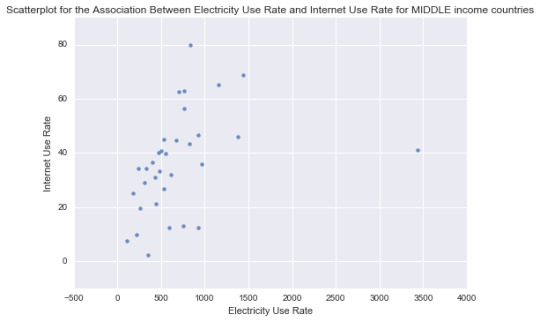
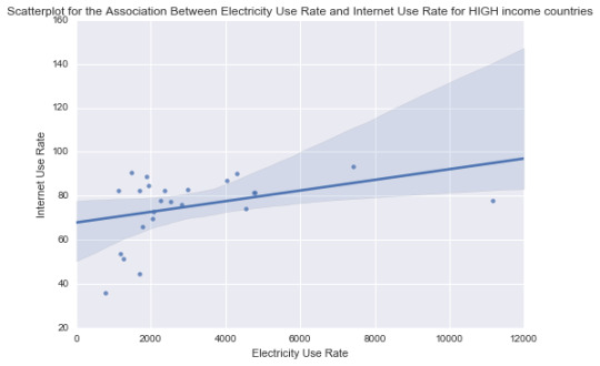
For the low income group the correlation between electricity use and Internet use rate is 1.0 and with a significant P value of 0.0. For the middle income countries, the association between Electricity use and Internet use rate is 0.36 and a P value, 0.038. not significant and finally among high income countries the correlation coefficient is 0.378, with a large P value of 0.0689 suggesting that the association between Electricity use and Internet use rate is not significant for high income countries. The significant/not-significant relationships is better visualized when each income group was mapped onto the associated scatter plots for each income group. Estimating a line of best fit within each scatter plot shows the positive association between Electricity use and Internet use rate among the low and high income countries. And almost no relationship between these variables in the middle income countries.
In conclusion, the moderator variable, income group variable interacts differently between the association of electricity use and internet rate. Therefore, the association between electricity use and internet use rate may not implies causation.

0 notes
Text
Below is the code that I used for this Pearson correlation Test:
import pandas as pd
import numpy as np import scipy.stats import seaborn as sb import matplotlib.pyplot as plt
ad = pd.read_csv(‘research_data.csv’, low_memory=False)
#bug fix for display formats to avoid run time errors - put after code for loading data above pd.set_option('display.float_format’, lambda x:’%f’%x)
#Set PANDAS to show all columns in DataFrame pd.set_option('display.max_columns’, None)
#Set PANDAS to show all rows in DataFrame pd.set_option('display.max_rows’, None)
# new code setting variables you will be working with to numeric
ad['incomeperperson’] = pd.to_numeric(ad['incomeperperson’], errors='coerce’) ad['co2emissions’] = pd.to_numeric(ad['co2emissions’], errors='coerce’) ad['oilperperson’] = pd.to_numeric(ad['oilperperson’], errors='coerce’) ad['relectricperperson’] = pd.to_numeric(ad['relectricperperson’], errors='coerce’) ad['urbanrate’] = pd.to_numeric(ad['urbanrate’], errors='coerce’) ad['internetuserate’] = pd.to_numeric(ad['internetuserate’], errors='coerce’)
print('Checking the column types:\n’) print(ad.dtypes)
data_clean = ad[['incomeperperson’, 'co2emissions’ , 'oilperperson’ , 'relectricperperson’ , 'urbanrate’ , 'internetuserate’]].dropna()
scat1 = sb.regplot(x=“incomeperperson”, y=“co2emissions”, fit_reg=True, data=ad) plt.xlabel('Income per Person’) plt.ylabel('Level of Co2 Pollution’) plt.title('Scatterplot for the Association Between Income per Person and Level of Co2 Pollution’) plt.show()
print(’\n’)
print ('Association Between Income per Person and Level of Co2 Pollution’) print (scipy.stats.pearsonr(data_clean['incomeperperson’], data_clean['co2emissions’]))
print(’\n’)
scat2 = sb.regplot(x=“incomeperperson”, y=“oilperperson”, fit_reg=True, data=ad) plt.xlabel('Income per Person’) plt.ylabel('Oil Use Rate’) plt.title('Scatterplot for the Association Between Income per Person and Oil Use Rate’) plt.show()
print(’\n’)
print ('Association between Income per Person and Oil Use Rate’) print (scipy.stats.pearsonr(data_clean['incomeperperson’], data_clean['oilperperson’]))
scat3 = sb.regplot(x=“incomeperperson”, y=“relectricperperson”, fit_reg=True, data=ad) plt.xlabel('Income per Person’) plt.ylabel('Eletricity Use Rate’) plt.title('Scatterplot for the Association Between Income per Person and Electricity Use Rate’) plt.show()
print(’\n’)
print ('Association between Income per Person and Electricity Use Rate’) print (scipy.stats.pearsonr(data_clean['incomeperperson’], data_clean['relectricperperson’]))
scat4 = sb.regplot(x=“incomeperperson”, y=“internetuserate”, fit_reg=True, data=ad) plt.xlabel('Income per Person’) plt.ylabel('Internet Use Rate’) plt.title('Scatterplot for the Association Between Income per Person and Internet Use Rate’) plt.show()
print(’\n’)
print ('Association between Income per Person and internetuserate’) print (scipy.stats.pearsonr(data_clean['incomeperperson’], data_clean['internetuserate’]))
scat5 = sb.regplot(x=“co2emissions”, y=“oilperperson”, fit_reg=True, data=ad) plt.xlabel('Level of Co2 Pollution’) plt.ylabel('Oil Use Rate’) plt.title('Scatterplot for the Association Between Level of Co2 Pollution and Oil Use Rate’) plt.show()
print(’\n’)
print ('Association between Level of Co2 Pollution and Oil Use Rate’) print (scipy.stats.pearsonr(data_clean['co2emissions’], data_clean['oilperperson’]))
scat6 = sb.regplot(x=“co2emissions”, y=“relectricperperson”, fit_reg=True, data=ad) plt.xlabel('Level of Co2 Pollution’) plt.ylabel('Electricity Use Rate’) plt.title('Scatterplot for the Association Between Level of Co2 Pollution and Electricity Use Rate’) plt.show()
print(’\n’)
print ('Association between Level of Co2 Pollution and Electricity Use Rate’) print (scipy.stats.pearsonr(data_clean['co2emissions’], data_clean['relectricperperson’]))
scat7 = sb.regplot(x=“urbanrate”, y=“internetuserate”, fit_reg=True, data=ad) plt.xlabel('Urban Use Rate’) plt.ylabel('Internet Use Rate’) plt.title('Scatterplot for the Association Between Urban Use Rate and Internet Use Rate’) plt.show()
print(’\n’)
print ('Association between Urban Use Rate and internetuserate’) print (scipy.stats.pearsonr(data_clean['urbanrate’], data_clean['internetuserate’]))
scat8 = sb.regplot(x=“relectricperperson”, y=“internetuserate”, fit_reg=True, data=ad) plt.xlabel('Electricity Use Rate’) plt.ylabel('Internet Use Rate’) plt.title('Scatterplot for the Association Between Electricity Use Rate and Internet Use Rate’) plt.show()
print(’\n’)
print ('Association between Electricity Use Rate and internetuserate’) print (scipy.stats.pearsonr(data_clean['relectricperperson’], data_clean['internetuserate’]))
Output/Interpretation
Association Between Income per Person and Level of Co2 Pollution
(0.31035401094147719, 0.016744622032815043)
Association between Income per Person and Oil Use Rate
(0.6570868144442028, 1.5825198974985358e-08)
Association between Income per Person and Electricity Use Rate
(0.67142450705471168, 5.8697009282903599e-09)
Association between Income per Person and internet use rate
(0.82460640750075942, 1.0003780006157626e-15)
Association between Level of Co2 Pollution and Oil Use Rate
(0.17375110868005739, 0.18814444744418543)
Association between Level of Co2 Pollution and Electricity Use Rate
(0.16994565558372737, 0.1981530500097772)
Association between Urban Use Rate and internetuserate
(0.59966996098570002, 5.1963769317132386e-07)
Association between Electricity Use Rate and internet use rate
(0.61178097012407806, 2.6354315417314502e-07)
Interpretation
I compiled the table above to illustrate and summarize the form, direction and strength of the Pearson correlation among the variables. It is clear that income correlates very well with internet use, while income correlates moderately with oil use and electricity use. Urban rate and electricity also correlates moderately with internet use. The association between income and level of pollution(co2 emission) is week.In conclusion the higher the income level of individuals there more the use the… actions
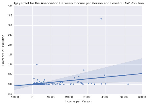
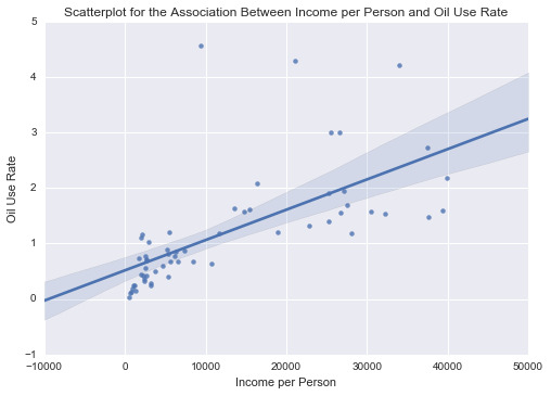
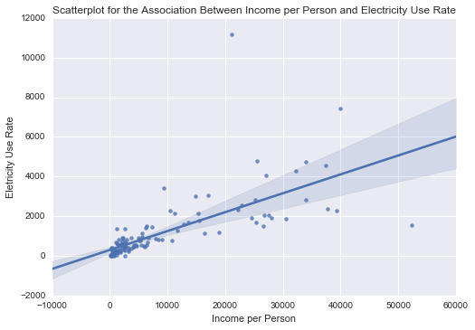
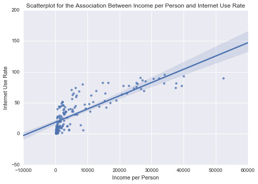
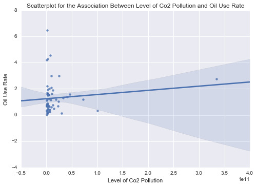
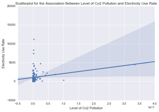
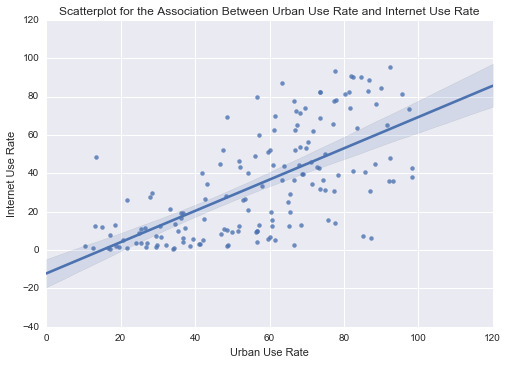
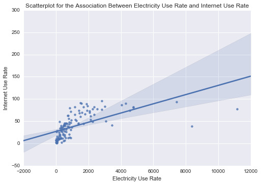

0 notes
Text
I started with a coding of comparison between Elevels (co2 emission levels) and oil use rate (oilperprson). I run chi-square independence test between the two categorical variables. The explanatory variable, Elevels was slit into 4 groups (close to quartiles). The response variable oil use rate was also grouped into 4.
# recode missing values to python missing (NaN)
ad[‘oilperperson’]=ad['oilperperson’].replace(1.5, np.nan)
ad['relectricperperson’]=ad['relectricperperson’].replace(1173, np.nan)
# cut co2 emissions into groups).
ad['co2eperperson’] = ad['co2emissions’] / 1000000000
ad['Elevels’] = pd.cut(ad['co2eperperson’],[0.0,0.35,1.90,18.50,3342.2], labels=[0.0,0.35,1.90,18.50])
# cut oil per person into groups))
ad['oiluse’]=pd.cut(ad['oilperperson’],[0.0,0.5,1,1.6,12.3], labels=[0.0,0.5,1,1.6])
# cut electricity use into groups).
ad['electricuse’]=pd.cut(ad['relectricperperson’],[0,203.6,579.1,1491.1,11154.76], labels=[0,203.6,579.1,1491.1])
I also displayed contingency table of observed counts, and calculate column percentages of this table.
I eventually run a chi-square test, displayed the result graphically, and analyzed post hoc
paired comparisons for the values of the explanatory variable. I did six comparisons because the explanatory variable has four levels. Below is part of the post hoc chi square test:
recode2= { 0:0 , 0.35:0.35}
sub1['COMP0v0.35’]= sub1['Elevels’].map(recode2)
# contingency table of observed counts
ct2=pd.crosstab(sub1['oiluse’], sub1['COMP0v0.35’])
print (ct2)
print(’\n’)
# column percentages
colsum=ct2.sum(axis=0)
colpct=ct2/colsum
print(colpct)
print(’\n’)
print ('chi-square value, p value, expected counts’)
cs2= scipy.stats.chi2_contingency(ct2)
print (cs2)
print(’\n’)
recode3= { 0:0 , 1.9:1.9}
sub1['COMP0v1.9’]= sub1['Elevels’].map(recode3)
# contingency table of observed counts
ct3=pd.crosstab(sub1['oiluse’], sub1['COMP0v1.9’])
print (ct3)
print(’\n’)
# column percentages
colsum=ct3.sum(axis=0)
colpct=ct3/colsum
print(colpct)
print(’\n’)
print ('chi-square value, p value, expected counts’)
cs3= scipy.stats.chi2_contingency(ct3)
print (cs3)
print(’\n’)
I coded the pvalue: print(0.05/6).
Output
Chi square test and graph
Elevels 0.000000 0.350000 1.900000 18.500000
oiluse
0.000000 0 4 9 2
0.500000 1 5 9 1
1.000000 0 3 6 6
1.600000 0 3 10 2
Elevels 0.000000 0.350000 1.900000 18.500000
oiluse
0.000000 0.000000 0.266667 0.264706 0.181818
0.500000 1.000000 0.333333 0.264706 0.090909
1.000000 0.000000 0.200000 0.176471 0.545455
1.600000 0.000000 0.200000 0.294118 0.181818
chi-square value, p value, expected counts
(10.035324569221626, 0.34763306474571631, 9, array([[ 0.24590164, 3.68852459, 8.36065574, 2.70491803],
[ 0.26229508, 3.93442623, 8.91803279, 2.8852459 ],
[ 0.24590164, 3.68852459, 8.36065574, 2.70491803],
[ 0.24590164, 3.68852459, 8.36065574, 2.70491803]]))
The chi-square value, p value, expected counts
(10.035324569221626, 0.34763306474571631
As the p-value = 0.35 is greater than 0.05, I accept the null hypothesis but it appears from the graph that there is a dependence between oil use rate and emission levels. All the empty spaces (data gaps) within the oilperperson and co2emission were replaces with their respective average values of the datasets. This may have created a coincidence of dependences as seen from the graphs.
The output of the post hoc test is provided below:
OMP0v0.35 0.000000 0.350000
oiluse
0.000000 0 4
0.500000 1 5
1.000000 0 3
1.600000 0 3
COMP0v0.35 0.000000 0.350000
oiluse
0.000000 0.000000 0.266667
0.500000 1.000000 0.333333
1.000000 0.000000 0.200000
1.600000 0.000000 0.200000
chi-square value, p value, expected counts
(1.7777777777777777, 0.61978263858771876, 3, array([[ 0.25 , 3.75 ],
[ 0.375 , 5.625 ],
[ 0.1875, 2.8125],
[ 0.1875, 2.8125]]))
COMP0v1.9 0.000000 1.900000
oiluse
0.000000 0 9
0.500000 1 9
1.000000 0 6
1.600000 0 10
COMP0v1.9 0.000000 1.900000
oiluse
0.000000 0.000000 0.264706
0.500000 1.000000 0.264706
1.000000 0.000000 0.176471
1.600000 0.000000 0.294118
chi-square value, p value, expected counts
(2.5735294117647061, 0.4621490922824335, 3, array([[ 0.25714286, 8.74285714],
[ 0.28571429, 9.71428571],
[ 0.17142857, 5.82857143],
[ 0.28571429, 9.71428571]]))
COMP0v18.5 0.000000 18.500000
oiluse
0.000000 0 2
0.500000 1 1
1.000000 0 6
1.600000 0 2
COMP0v18.5 0.000000 18.500000
oiluse
0.000000 0.000000 0.181818
0.500000 1.000000 0.090909
1.000000 0.000000 0.545455
1.600000 0.000000 0.181818
chi-square value, p value, expected counts
(5.4545454545454559, 0.14138272114763559, 3, array([[ 0.16666667, 1.83333333],
[ 0.16666667, 1.83333333],
[ 0.5 , 5.5 ],
[ 0.16666667, 1.83333333]]))
COMP0.35v1.9 0.350000 1.900000
oiluse
0.000000 4 9
0.500000 5 9
1.000000 3 6
1.600000 3 10
COMP0.35v1.9 0.350000 1.900000
oiluse
0.000000 0.266667 0.264706
0.500000 0.333333 0.264706
1.000000 0.200000 0.176471
1.600000 0.200000 0.294118
chi-square value, p value, expected counts
(0.55060331825037689, 0.90764144837111072, 3, array([[ 3.97959184, 9.02040816],
[ 4.28571429, 9.71428571],
[ 2.75510204, 6.24489796],
[ 3.97959184, 9.02040816]]))
COMP0.35v18.5 0.350000 18.500000
oiluse
0.000000 4 2
0.500000 5 1
1.000000 3 6
1.600000 3 2
COMP0.35v18.5 0.350000 18.500000
oiluse
0.000000 0.266667 0.181818
0.500000 0.333333 0.090909
1.000000 0.200000 0.545455
1.600000 0.200000 0.181818
chi-square value, p value, expected counts
(4.012929292929293, 0.26007138020944137, 3, array([[ 3.46153846, 2.53846154],
[ 3.46153846, 2.53846154],
[ 5.19230769, 3.80769231],
[ 2.88461538, 2.11538462]]))
COMP1.9v18.5 1.900000 18.500000
oiluse
0.000000 9 2
0.500000 9 1
1.000000 6 6
1.600000 10 2
COMP1.9v18.5 1.900000 18.500000
oiluse
0.000000 0.264706 0.181818
0.500000 0.264706 0.090909
1.000000 0.176471 0.545455
1.600000 0.294118 0.181818
chi-square value, p value, expected counts
(5.9996353913466223, 0.11162796544563411, 3, array([[ 8.31111111, 2.68888889],
[ 7.55555556, 2.44444444],
[ 9.06666667, 2.93333333],
[ 9.06666667, 2.93333333]]))
Adjusted p value
0.008333333333333333
Among the six comparisons analyzed, all the pvalues are greater than 0.0083 (0.05/6). I conclude that the oil use rate and co2 emission levels (Elevels) are not independent and that the results are inconclusive as at this point.
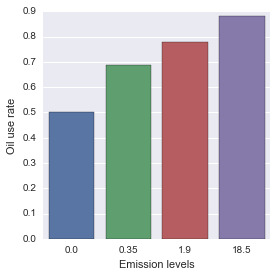
0 notes
Text
DataAnalysisTools-W1-Assignment
The variable “co2eperperson” shows total co2 emissions emitted per person between 1975 and 2006. The variable is calculated by the total co2 emissions divided by the population of each country.
The variable “tropics” the tropic zones from the Equator, measured in degrees of each country’s centroid which is the value of the corresponding latitude.
The variable “Ilevel” indicates income level per person and the variable “PLevel” indicates the level of co2 emitted/polluted per person.
In this Data Analysis Tools, assignment, I intend to use the Analysis of Variance (ANOVA) to examine the association between the co2 emissions per person (quantitative variable) and the tropical zones (categorical explanatory) and Ilevels (categorical explanatory).
The categorical variable Ilevel representing income levels is divided into
5 categories – Very low income, Low income, middle income, high income and very high income.
The categorical variable Plevel is divided into 3 categories- low pollution, medium pollution and high pollution.
The null hypothesis is that the rate co2 emissions emitted per person does not depend on tropical zone. The alternative hypothesis is that co2 emissions emitted per person depends on tropical zone.
Results
counts for tropics
tropic_of_cancer 21
tropic_of_capricon 55
others 78
Name: tropics, dtype: int64
percentages for tropics
tropic_of_cancer 0.136364
tropic_of_capricon 0.357143
others 0.506494
Name: tropics, dtype: float64
OLS Regression Results
==============================================================================
Dep. Variable: co2eperperson R-squared: 0.178
Model: OLS Adj. R-squared: 0.167
Method: Least Squares F-statistic: 15.95
Date: Fri, 21 Oct 2016 Prob (F-statistic): 5.40e-07
Time: 10:57:18 Log-Likelihood: -1081.1
No. Observations: 150 AIC: 2168.
Df Residuals: 147 BIC: 2177.
Df Model: 2
Covariance Type: nonrobust
====================================================================================================
coef std err t P>|t| [95.0% Conf. Int.]
—————————————————————————————————-
Intercept 36.8756 71.966 0.512 0.609 -105.346 179.097
C(tropics)[T.tropic_of_capricon] 27.9772 85.037 0.329 0.743 -140.075 196.029
C(tropics)[T.others] 323.6721 81.303 3.981 0.000 162.998 484.346
==============================================================================
Omnibus: 100.488 Durbin-Watson: 1.944
Prob(Omnibus): 0.000 Jarque-Bera (JB): 540.017
Skew: 2.555 Prob(JB): 5.46e-118
Kurtosis: 10.765 Cond. No. 5.70
==============================================================================
Warnings:
[1] Standard Errors assume that the covariance matrix of the errors is correctly specified.
means for co2eperperson by tropical zones
co2eperperson
tropics
tropic_of_cancer 36.875606
tropic_of_capricon 64.852816
others 360.547665
standard deviations for co2eperperson by tropical zones
co2eperperson
tropics
tropic_of_cancer 55.782929
tropic_of_capricon 159.083193
others 441.356848
OLS Regression Results
==============================================================================
Dep. Variable: co2eperperson R-squared: 0.590
Model: OLS Adj. R-squared: 0.579
Method: Least Squares F-statistic: 52.55
Date: Fri, 21 Oct 2016 Prob (F-statistic): 2.33e-27
Time: 10:57:18 Log-Likelihood: -1032.2
No. Observations: 151 AIC: 2074.
Df Residuals: 146 BIC: 2089.
Df Model: 4
Covariance Type: nonrobust
==========================================================================================
coef std err t P>|t| [95.0% Conf. Int.]
——————————————————————————————
Intercept 8.4456 41.803 0.202 0.840 -74.171 91.062
C(Ilevel)[T.LowI] 103.7053 48.012 2.160 0.032 8.817 198.594
C(Ilevel)[T.MiddleI] 710.7761 83.605 8.502 0.000 545.543 876.009
C(Ilevel)[T.highI] 804.1579 78.206 10.283 0.000 649.597 958.719
C(Ilevel)[T.VeryHighI] 826.2056 110.599 7.470 0.000 607.623 1044.788
==============================================================================
Omnibus: 83.828 Durbin-Watson: 1.677
Prob(Omnibus): 0.000 Jarque-Bera (JB): 545.022
Skew: 1.901 Prob(JB): 4.47e-119
Kurtosis: 11.495 Cond. No. 7.90
==============================================================================
Warnings:
[1] Standard Errors assume that the covariance matrix of the errors is correctly specified.
means for co2eperperson by Income levels
co2eperperson
Ilevel
VerylowI 8.445616
LowI 112.150866
MiddleI 719.221718
highI 812.603548
VeryHighI 834.651257
standard deviations for co2eperperson by Income levels
co2eperperson
Ilevel
VerylowI 10.350549
LowI 122.609107
MiddleI 574.105151
highI 429.621026
VeryHighI 560.362982
Multiple Comparison of Means - Tukey HSD, FWER=0.05
========================================================
group1 group2 meandiff lower upper reject
——————————————————–
LowI MiddleI 607.0709 396.7032 817.4385 True
LowI VeryHighI 722.5004 432.2353 1012.7655 True
LowI VerylowI -103.7053 -236.3263 28.9158 False
LowI highI 700.4527 506.5765 894.3289 True
MiddleI VeryHighI 115.4295 -230.9776 461.8366 False
MiddleI VerylowI -710.7761 -941.7142 -479.838 True
MiddleI highI 93.3818 -177.4171 364.1807 False
VeryHighI VerylowI -826.2056 -1131.708 -520.7033 True
VeryHighI highI -22.0477 -358.6949 314.5995 False
VerylowI highI 804.1579 588.1352 1020.1807 True
——————————————————–
The ANOVA depicted that the F-statistic is 15.95, and the p-value is 5.4e-7. Therefore, the null hypothesis must be rejected. The error of committing type 1 error is insignificantly small.
The rate of co2 emitted per person depends on tropical zones. More co2 is emitted in the zone outside the 2 tropics.
Considering the Post hoc comparisons of mean values of the co2 emitted per person pairs by the pairs 5 income level categories shows those means are significantly different for the income level e zone pairs LowI-MiddleI, LowI-VeryHighI, LowI-HighI, MiddleI-VeryL and VeryHighI-VeryLowI.
0 notes
Text
Week-4 Assignment
I plotted the relationship between variables for visualization.
Below is the portion of the code I used to plots my graphs:
# Create a new variables
ad[‘co2eperperson’] = ad['co2emissions’] / ad['pop95’]
#create a form of a secondary variable to slip co2 emissions per person into polution levels (lowP, mediumP and highP)
ad['Plevel’] = pd.cut(ad['co2eperperson’],[1,660,1320,1980], labels=['lowP’,'mediumP’,'highP’])
#create a new variable to slit Income per person into lowI, mediumI and highI
ad['Ilevel’] = pd.cut(ad['incomeperperson’],[100,18000,35000,53000],labels=['lowI’, 'mediumI’, 'highI’])
#create a new variable to slip latitudes into tropics (tropic of cancer and tropic of capricon)
ad['tropics’] = pd.cut(ad['cen_lat’],[-23.5,0,23.5,75],labels=['tropic_of_cancer’, 'tropic_of_capricon’, 'others’])
ad['tropics’] = ad['tropics’].astype(“category”)
sb.factorplot(x='tropics’, y='co2eperperson’, data=ad,
kind=“bar”, ci=None, size=7)
plt.xlabel('Climate zones’)
plt.ylabel('Co2 per Person output rate’)
plt.show()
# Frequency distribution for the variable 'region’
print ('counts for tropics’)
c_tropics = ad['tropics’].value_counts(sort=False)
print (c_tropics)
print(’\n’)
print ('percentages for tropics’)
p_tropics = ad['tropics’].value_counts(sort=False,
normalize=True)
print (p_tropics)
print(’\n’)
sb.countplot(x='tropics’,data=ad)
plt.xlabel('Climate zones’)
plt.ylabel('Number of countries’)
plt.title('Distribution of Climatic Zones by Countries’)
plt.show()
sb.countplot(x='Plevel’,data=ad)
plt.xlabel('Climate zones’)
plt.ylabel('Number of countries’)
plt.title('Distribution of Pollutions Levels by Countries’)
plt.show()
#basic scatterplot: Q->Q
scat1 = sb.regplot(x=“incomeperperson”, y=“oilperperson”, data=ad)
plt.xlabel('Income per Person’)
plt.ylabel('Oil Consumption per Capita’)
plt.title('Scatterplot for the Association Between Income per Person and Oil consumption per Capita’)
plt.show()
scat2 = sb.regplot(x=“incomeperperson”, y=“co2emissions”, data=ad)
plt.xlabel('Income per Person’)
plt.ylabel('Co2 Emissions’)
plt.title('Scatterplot for the Association Between Income per Person and Co2 Emissions’)
plt.show()
scat3 = sb.regplot(x=“oilperperson”, y=“co2emissions”, data=ad)
plt.xlabel('Oil Consumption per Capita’)
plt.ylabel('Co2 Emissions’)
plt.title('Scatterplot for the Association Between Oil Consumption per Capita and Co2 Emissions’)
plt.show()
scat4 = sb.regplot(x=“incomeperperson”, y=“hivrate”, data=ad)
plt.xlabel('Income per Person’)
plt.ylabel('HIV Rate’)
plt.title('Scatterplot for the Association Between Income per Person and HIV Rate’)
plt.show()
# quartile split (use qcut function & ask for 4 groups - gives you quartile split)
print ('Income per person - 4 categories - quartiles’)
ad['INCOMEGRP4’]=pd.qcut(ad.incomeperperson, 4, labels=[“1=25th%tile”,“2=50%tile”,“3=75%tile”,“4=100%tile”])
c6 = ad['INCOMEGRP4’].value_counts(sort=False, dropna=True)
print (c6)
# bivariate bar graph C->Q
sb.factorplot(x='INCOMEGRP4’, y='hivrate’, data=ad, kind=“bar”, ci=None, size=7)
plt.xlabel('income group’)
plt.ylabel('mean HIV rate’)
c7= ad.groupby('INCOMEGRP4’).size()
print (c7)
result = ad.sort(['INCOMEGRP4’], ascending=[1])
print(result)
Output
counts for tropics
tropic_of_cancer 21
tropic_of_capricon 55
others 78
Name: tropics, dtype: int64
percentages for tropics
tropic_of_cancer 0.136364
tropic_of_capricon 0.357143
others 0.506494
Name: tropics, dtype: float64
Univariate graphs
Tropic of cancer has less number of countries.
Few countries have high level of pollution while more counttries pollute less.
Scatter plots
Interpretation
There is a strong positive relationship between income levels and oil consumption. This means the higher an individual income is the more oil he consumes, which is in line with my initial one of my initial hypothesis. This also implies richer countries consume more oil than poorer countries.
Interpretation
The slope of the regression is positive but concentrated at the bottom half of the plot indicating a weaker association between a person’s income and co2 emissions. This mean an individual’s carbon foot print depends on multiple factors including the income level of the person.
Interpretation
Similarly, the slope of the regression is positive but concentrated at the bottom half of the plot indicating a weaker association between a person’s oil consumption and co2 emissions. This mean an individual’s carbon foot print depends on multiple factors including the amount of oil he consumes.
Interpretation
The correlation between income person and HIV rates are not presented well in this graph although more HIV people appears to have low income.
Bivariate graphs
Interpretation
The correlation between HIV rate and income person is negative. This means the higher the HIV rate the lower the income per person. This implies low income countries are prone to HIV than richer countries.
The combined Co2 per person output rate in the Tropic of cancer and tropic of Capricorn is less than zones outside the tropics

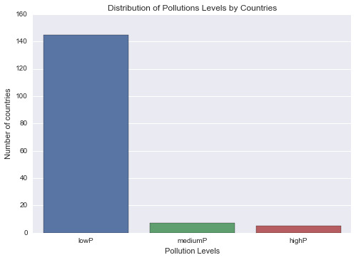
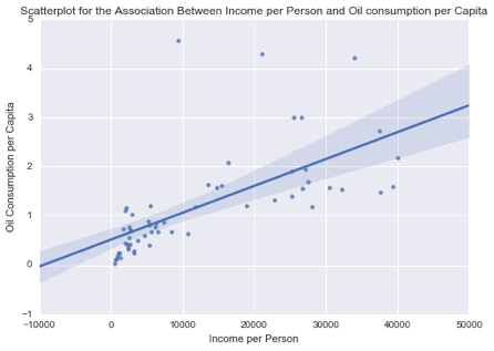
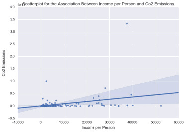
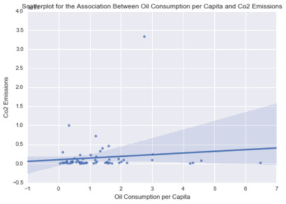
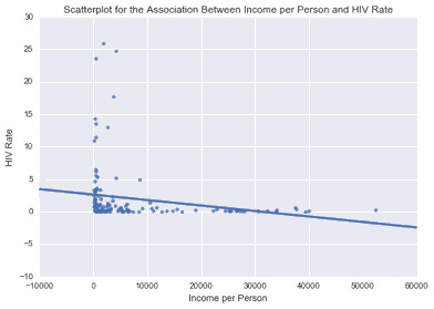
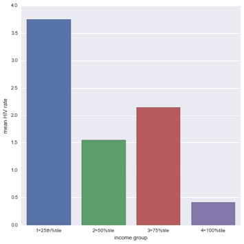
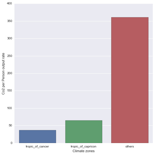
0 notes
Text
Output This graph is unimodal, with its highest pick at 0-20% of breast cancer rate. It seems to be skewed to the right as there are higher frequencies in lower categories than the higher categories. This graph is unimodal, with its highest pick at 0-1% of HIV rate. It seems to be skewed to the right as there are higher frequencies in lower categories than the higher categories. This graph is unimodal, with its highest pick at the median of 55-60% employment rate. It seems to be a symmetric distribution as there are lower frequencies in lower and higher categories. This graph plots the breast cancer rate vs. HIV rate for people with a high suicide rate. It shows that people with breast cancer are not infected with HIV. -------------------------------------------------------------------------------------------------------------------------------------------------------- import pandas as pd import numpy as np import seaborn as sb import matplotlib.pyplot as plt # load gapminder dataset data = pd.read_csv('gapminder.csv',low_memory=False) # lower-case all DataFrame column names data.columns = map(str.lower, data.columns) # bug fix for display formats to avoid run time errors pd.set_option('display.float_format', lambda x:'%f'%x) # setting variables to be numeric data['suicideper100th'] = data['suicideper100th'].convert_objects(convert_numeric=True) data['breastcancerper100th'] = data['breastcancerper100th'].convert_objects(convert_numeric=True) data['hivrate'] = data['hivrate'].convert_objects(convert_numeric=True) data['employrate'] = data['employrate'].convert_objects(convert_numeric=True) # display summary statistics about the data # print("Statistics for a Suicide Rate") # print(data['suicideper100th'].describe()) # subset data for a high suicide rate based on summary statistics sub = data[(data['suicideper100th']>12)] #make a copy of my new subsetted data sub_copy = sub.copy() # Univariate graph for breast cancer rate for people with a high suicide rate plt.figure(1) sb.distplot(sub_copy["breastcancerper100th"].dropna(),kde=False) plt.xlabel('Breast Cancer Rate') plt.ylabel('Frequency') plt.title('Breast Cancer Rate for People with a High Suicide Rate') # Univariate graph for hiv rate for people with a high suicide rate plt.figure(2) sb.distplot(sub_copy["hivrate"].dropna(),kde=False) plt.xlabel('HIV Rate') plt.ylabel('Frequency') plt.title('HIV Rate for People with a High Suicide Rate') # Univariate graph for employment rate for people with a high suicide rate plt.figure(3) sb.distplot(sub_copy["employrate"].dropna(),kde=False) plt.xlabel('Employment Rate') plt.ylabel('Frequency') plt.title('Employment Rate for People with a High Suicide Rate') # Bivariate graph for association of breast cancer rate with HIV rate for people with a high suicide rate plt.figure(4) sb.regplot(x="hivrate",y="breastcancerper100th",fit_reg=False,data=sub_copy) plt.xlabel('HIV Rate') plt.ylabel('Breast Cancer Rate') plt.title('Breast Cancer Rate vs. HIV Rate for People with a High Suicide Rate')
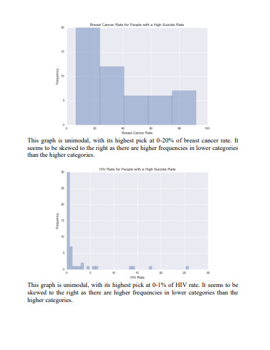
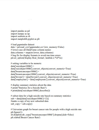
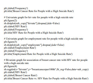
0 notes
