data-analytics-adagarzasing-blog

[data-analytics-adagarzasing-blog]

Assignment  4 - Test  a Logistical Regression Model.

For this study I ran two models to see results against to explanatory variables:

The first one is for explanatory variable ‘Race’ and whether this had a bearing on whether adolescents exhibited drinking and smoking behaviors more often or not. 

Code Using ‘Race’ as an explanatory variable

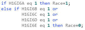
First I needed to code the Race variable (H1GI61A) in order to make this variable binary. Since most of the race questions were not answered, I had to separate the response based on the race of the respondent being “White” vs “Other. The code is as follows:

Results

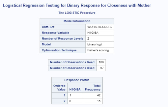
When we see the results for this code, there ware 42 responses equivalent to Race = White and “Other” with 15 responses. 

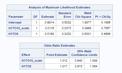
Based on the analysis of maximum likelihood estimates and the odds ratio -  after adjusting for potential confounding factors (H1TO15_scale - Number if Days Alcohol Consumed in Past 12 Month and H1TO5 - Number of Days where Cigarettes were Smoked in Past 30 Days) - the odds of adolescents consuming more cigarettes or alcohol are not statistically significant as both p values are greater than p.05 (p=.76, p=.47).

Code Using ‘Closness with Mother’ as an explanatory variable

Using my original explanatory variable - closeness with mother - the variable was collapsed as per code below. Any answers with  H1NM14_grouped=0 represent responses where the adolescent did not feel close to his/her biological non-resident mother. Whereas, any answers with  H1NM14_grouped=1, represent responses where the adolescent felt some degree of closeness with his/her biological non-resident mother.

Results 

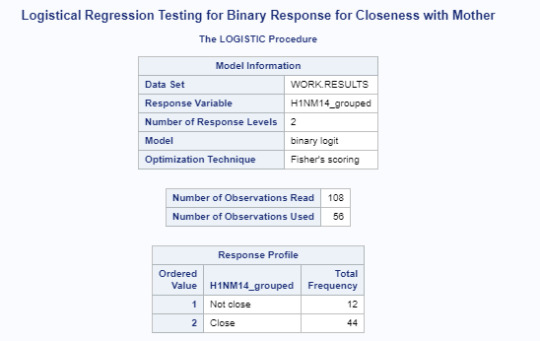
As the results table reflects above, there are 12 respondents in the surveyed population that do not feel close to their mother. 44 respondents feel close to their mother. 

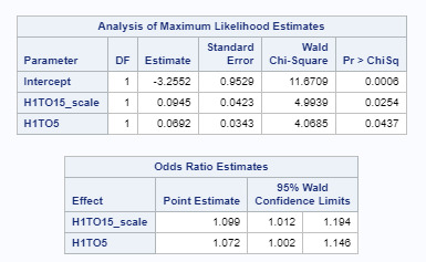
Based on the analysis of maximum likelihood estimates and the odds ratio -  after adjusting for potential confounding factors (number of cigarettes and number of alcoholic drinks consumed), the odds of consuming more alcoholic drinks is 1.1 times higher for participants that do not feel close to their biological non resident mother than those with greater degree of closeness. (OR=1.1, 95% CI = 1.01-1.20, p=.025). Number of cigarettes consumed was also significantly associated with how close the adolescent feels to his/her biological mother, such that the closer the bond between the adolescent and the mother the less likely to consume cigarettes (OR= 1.10, 95% CI=1.00-1.15, p=.044).

[data-analytics-adagarzasing-blog]

Assignment # 3 Week # 3- Test a Multiple Regression Model

In order to determine whether there are any other factors that might influence the amount of alcohol or cigarettes smoked in adolescents - other than their being close to their non-resident biological mother, I added another variable to the mix -  H1NM8 - Age When Living with Non-Res Bio Mother.

This is the age of when the adolescent last lived with his or her biological mother. 

Centering our new Variable

I added the new variable by creating a test data set and obtaining the mean of our variable before centering it. 

/*Finding the Mean*/

PROC MEANS DATA=ADASDATA.NEW; VAR  H1NM8; RUN;

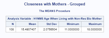
/* Centering our variable - Analysis Variable : H1NM8 Age When Living with Non-Res Bio Mother*/ 

Data mrnew; set adasdata.new; H1NM8_C=H1NM8-15.4907407; Run;

/* Verifying that the new variable is centred*/

PROC MEANS DATA=mrnew; VAR  H1NM8_C; RUN;

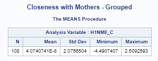
Introducing the newly centered variable

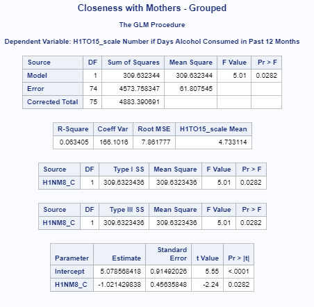
I used the PROC GLM procedure to model our newly centered variable against our response variables.

/*Using our newly centered variable in our regression analysis*/ proc glm; model H1TO15_scale = H1NM8_C/solution; run;

The polynomial regression plot was created with these variables in order to understand their impact.

/*Polynomial Regression - scatter plot with linear and quadratic regression line*/

proc sgplot;

reg x=H1NM8_C y=H1TO15_scale / lineattrs=(color=blue thickness=2) degree=1 clm;

reg x=H1NM8_C y=H1TO15_scale / lineattrs=(color=blue thickness=2) degree=2 clm; yaxis label="Number if Days Alcohol Consumed in Past 12 Months"; xaxis labeL="Age When Living with Non-Res Bio Mother"; run;

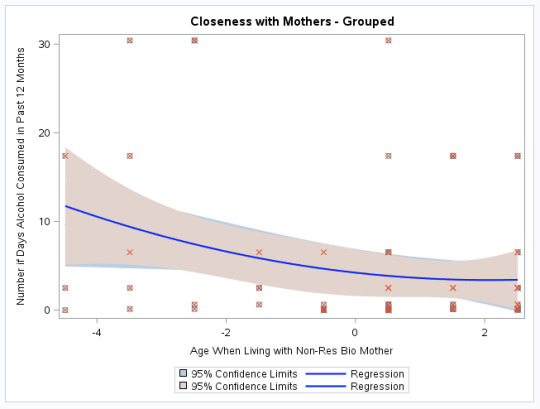
Regression Diagnostic Plots

Finally in order to test our multiple regression model, the following code was used to create a series of graphs that would allows to understand the relationship between our response and our new explanatory variable: 

/*Testing our regression model*/

PROC GLM; MODEL H1TO15_scale = H1NM8_C/solution CLPARM; RUN;

PROC GLM; MODEL H1TO5 H1TO15_scale = H1NM8_C H1NM8_C * H1NM8_C/solution CLPARM; RUN;

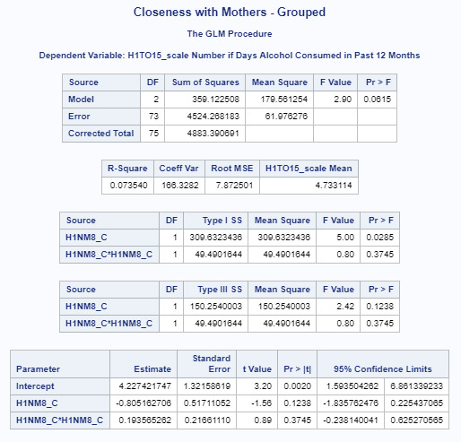
After adjusting for potential confounding factors - age of the adolescent when biological mother still lived with them and the number of days Alcohol consumed in the past 12 months, it is seen that this explanatory variable (Beta=.07, p=.3745) it is not significantly associated with the adolescent consuming alcohol or cigarettes. 

PLOTS

ods graphics on;

PROC GLM PLOTS(UNPACK)=ALL; MODEL H1TO15_scale = H1NM8_C H1NM8_C * H1NM8_C/solution CLPARM; OUTPUT RESIDUAL=RES STUDENT=STDRES OUT=RESULTS; RUN;

ods graphics off;

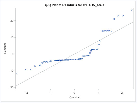
The QQ Plot Interpretation

The non linearity of the points in the graph below indicate a departure from normality. There is some curvature towards the middle of the graph with slope increasing from left to right, which means that maybe another type of distribution testing (e.i. lognormal distribution) can be used to obtain a better fit than normal distribution. Also, it is visible that as the graph slopes towards the right, there is somewhat of a staircase pattern which might be due to the data being discrete or rounding.

Standardized Residual Plot Interpretation 

Using our new quadratic variable, the code to obtain the standardized residuals plot is as follows:

PROC GPLOT; LABEL STDRES="Standardized Residual" H1NM8_C=H1NM8_C; plot stdres*H1NM8_C/vref=0; ods graphics off;

The graph results are below, which shows that the 

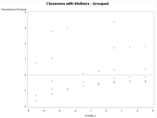
Mean residual is zero. The data does not seem to be normalized as it does not follow the shape of the standard deviation. While most of the values are between +2/-2, there continues to be be some outliers which means that there might be other variables that are not being taken into consideration for our analysis. More over, a lot of the values are negative and this might also mean that we need to add more explanatory variables to our analysis.  

Outlier and Leverage Diagnostics

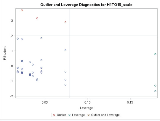
Interpreting For the current analysis, there are only 3 outlying observations above the horizontal line at the +2 mark. This means that these observations have large residuals. Most of the observations on the left lower quadrant fall close to the mean. However, there are some observations within this quadrant that are quite far away from the mean. There are also three points that could influence the direction of the slop on the right bottom quadrant. 

[data-analytics-adagarzasing-blog]

Assignment # 2 - Test a Basic Linear Regression Model

Centering the Variable

The following variable has been centered:

/* H1NM14 has been collapsed to dichotomy: Close vs Not close. Additionally, since this is a categorical explanatory variable, then a response of no being close to their biological non-resident mother is set to zero, while a response of feeling close to their biological non-resident mother is set to one */

 if H1NM14 in (1,2) then H1NM14_grouped=0;  else if H1NM14 in (3,4,5) then H1NM14_grouped=1;  else call missing(H1NM14_grouped);

PROC GLM

The PROC GLM code was used below:

title 'Closeness with Mothers - Grouped'; proc glm data = adasdata.new;  class H1NM14_grouped;  model H1TO5 H1TO15_scale = H1NM14_grouped / SS3;  manova h = H1NM14_grouped; run;

Results

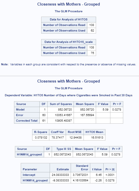
For our dependent variable, H1TO5 Number of Days where Cigarettes were Smoked in Past 30 Days, the F=5.09 and p=0.0278 which is less than alpha=0.05.

This tells us that we can reject the null hypothesis and conclude that closeness with biological non-resident mother is significantly associated with alcohol consumption in adolescents.

The beta sub one value here is -9.38 and the beta sub zero value is 24.08. So we now know that our equation for the best fit line of this graph, is Cigarette Consumption = -24.08 + (9.38) * H1TO5 Number of Days where Cigarettes were Smoked in Past 30 Days.

The R-Square value of .08 shows the proportion of the variance in the response variable that can be explained by the explanatory variable. Meaning, that this model accounts for 8% of the variability we see in our response variable H1TO5 Number of Days where Cigarettes were Smoked in Past 30 Days . 

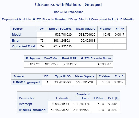
Similarly, for dependent variable  H1TO15_scale Number if Days Alcohol Consumed in Past 12 Months, F=10.58 and p-0.0017 which is considerably less than alpha=0.05.

This tells us that we can reject the null hypothesis and conclude that closeness with biological non-resident mother is significantly associated with cigarette consumption in adolescents.

The beta sub one value here is -6.85 and the beta sub zero value is 9.96. So we now know that our equation for the best fit line of this graph, is Fr= -9.96 + (6.85) * H1TO15_scale Number if Days Alcohol Consumed in Past 12 Months .

The R-Square value of .13 shows the proportion of the variance in the response variable that can be explained by the explanatory variable. Meaning, that this model accounts for 13% of the variability we see in our response variable  H1TO15_scale Number if Days Alcohol Consumed in Past 12 Months .

[data-analytics-adagarzasing-blog]

Writing About Your Data

Sample

The sample was drawn from The National Longitudinal Study of Adolescent Health (AddHealth) Waive 1. This is a nationally representative sample of adolescents in grades 7 through 12 in the US in the 1994–95 school year. Participants (N=6504) responded to questions related to factors that may influence adolescents’ health and risk behaviors, including personal traits, families, friendships, romantic relationships, peer groups, schools, neighborhoods, and communities. The AddHealth included a sampling of multiple nationalities such as Black, Hispanics, Pacific Asians,  Latino, White and Native American population of adolescents.  

The data analytic sample for this analysis includes participants 11 to 19 years of age who reported risky behaviors and provided responses to whether these adolescents felt close to their non-resident  biological mother.

Procedure

Wave I encompasses all data collection between 1994 and 1995. The primary sampling frame for Add Health is a database collected by Quality Education Data, Inc. Systematic sampling methods and implicit stratification ensure that the 80 high schools selected are representative of US schools with respect to region of country, urban city, size, type, and ethnicity.  Seventy-nine percent of all sampled students in all of the groups participated in Wave I of the in-home phase of the survey (20,745). Each school that declined to participate was replaced by a school within the stratum. Participating high schools helped to identify feeder schools—that is, schools that included a 7th grade and sent at least five graduates to that high school. School size varied from fewer than 100 students to more than 3,000 students. The communities were located in urban, suburban, and rural areas of the country. Each school administration occurred on a single day within one 45- to 60- minute class period. Add Health completed in-school questionnaires from over 90,000 students.

All students who completed the In-School Questionnaire plus those who did not complete a questionnaire but were listed on a school roster were eligible for selection into the core in-home sample.Students in each school were stratified by grade and sex. About 17 students were randomly chosen from each stratum so that a total of approximately 200 adolescents were selected from each of the 80 pairs of schools. A total core sample of 12,105 adolescents was interviewed.

A parent, usually the resident mother, also completed a 30- minute op-scan interviewer-assisted interview. Over 85 percent of the parents of participating adolescents completed the parental interview in the first wave.

Measures

The response variable used for this analysis was H1TO15_scale=“Number of Days Alcohol Consumed in Past 30 Days" found in the Section 28 of the code book – however the variable was scaled in order to represent number of days alcohol was consumed in the past 30 days (versus in the past 12 months). Based on a set of 6504 records in the code book, H1TO15 has 76 observations

As well, the explanatory variable of H1NM14="Closeness with Non-Res Bio Mother" – found in section 15 of the code book – was collapsed in order to make the variable dichotomous (provide a yes/no answer). Based on this management of the variable 102 observations were found.

Based on the results produced, it is determined that there is a statistically significant weak negative correlation between H1NM14_grouped and H1TO15_scale. This shows that it is unlikely that the negative relationship between the two variables would be due to chance alone and that amount of alcohol consumption can be affected by whether an adolescent feels closer to their non-resident biological mother - the close the adolescent feels to their non-resident biological mother, the less he or she is likely to consume alcohol.

[data-analytics-adagarzasing-blog]

Testing a Potential Moderator

Summary

Thus far, i have been analyzing the effects of the perceived closeness that an adolescent has with his/her non-resident biological mother and the frequency of alcohol consumption. Based on or correlation analysis, there is a negative relationship between these variables, were the closer the adolescent is to his non-resident biological mother, the lest he/she is inclined to consume alcohol. 

For this exercise, the moderator (third variable) chosen for my analysis is race of the adolescent. 

There are 5 possible races the adolescent can choose from:

H1GI6A - White; H1GI6B - African America ; H1GI6C-Native American; H1GI6D; Asian or Pacific Islander; H1GI6E - Other. 

For the purposes of our analysis this variable has been collapsed into a two level variable as the number of responses for each variable would not be able to provide a significant statistical interaction. 

Because the moderator variable only has two levels, there is no need for a post hoc test.

Moderator Variable

The code for the introduction of the new collapsed variable is as follows:

if H1GI6A eq 1 then Race=1;  else if H1GI6B eq 1 or          H1GI6C eq 1 or          H1GI6D eq 1 or          H1GI6E eq 1 then Race=0;

The code below will ensure that only answers of ‘yes’ or ‘no’ for each of the variable will be included in the analysis:

 if H1GI6A not in(0,1) then call missing(H1GI6A);  if H1GI6B not in(0,1) then call missing(H1GI6B);  if H1GI6C not in(0,1) then call missing(H1GI6C);  if H1GI6D not in(0,1) then call missing(H1GI6D);  if H1GI6E not in(0,1) then call missing(H1GI6E);

PROC REG Code

The analysis tool used in this exercise is PROC REG, to do regression analysis. The code to analyze the impact of race on the consumption of alcohol for those adolescents that are or aren’t close to their non reside biological mother is:

proc reg data=adasdata.new;

 model H1TO15_scale = H1NM14_grouped; run;

proc reg data=adasdata.new;  model H1TO15_scale = H1NM14_grouped race; run;

PROC REG Results

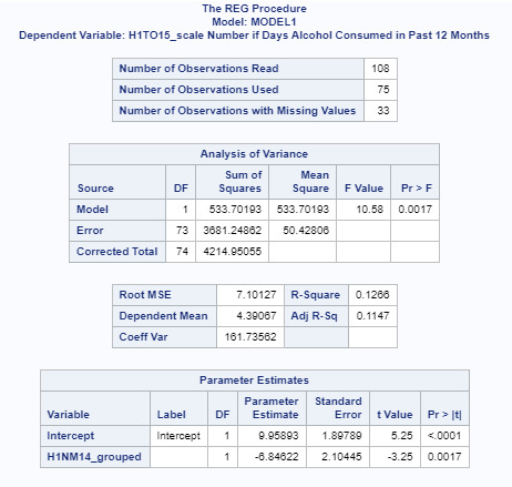
First, we can see that the p value for the analysis of variance is statistically significant between variables H1NM14_grouped and H1TO15_scale (p=0.0017). 

When we introduce the ‘race’ variable, the results are as follows:

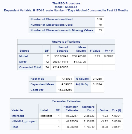
The results above show that while the p=value for H1NM14_grouped is statistically significant(p=0.0019), we see that when ‘race’ is factored in, the p value is quite high (p=0.9641). 

Therefore, we conclude that race is not a moderator between the level of alcohol consumption for adolescents whether they feel close to their non-resident biological mother or not. 

[data-analytics-adagarzasing-blog]

Correlation Coefficient

For this assignment, I will use H1NM14_grouped in order to collapse responses to two levels and show the relationship to H1TO15.

Code for H1NM14 and Pearson Correlation:

H1NM14

/*Collapse H1NM14 to dichotomy: Close vs Not close*/

 if H1NM14 in (1,2) then H1NM14_grouped=0;  else if H1NM14 in (3,4,5) then H1NM14_grouped=1;  else call missing(H1NM14_grouped);

Pearson Correlation

Title 'Correlation Procedure'; proc corr data=adasdata.new; run;

ods graphics on; title 'Closeness with Mother';

proc corr data=adasdata.new plots=matrix(histogram);

  var H1NM14_grouped H1TO15_scale; run;

ods graphics off;

PROC CORR Results

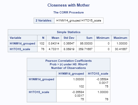
Based on the results produced, we can see there is a weak negative correlation between H1NM14_grouped and H1TO15_scale (r=-0.35584). Since p=0.0017, this is statistically significant which means that it is unlikely that the negative relationship between the two variables would be due to chance alone.

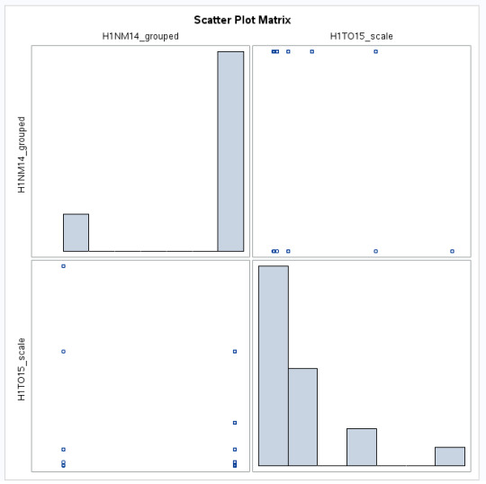
Scatter Plot Results

Predicting Variability

If we calculate r^2 (-0.35584)^2, we get 0.1266221056, or 0.13. This mean that if we know how close an adolescent is to his/her biological non-resident mother, we can predict 13% of the variability we will see in the number of alcoholic drinks consumed over a 30 day period of time. This also means that we do not know the other 87% of the variability. 

[data-analytics-adagarzasing-blog]

Running a Chi-Square Test of Independence

The two variables to be used for the Chi-Square test of indpendance are: H1NM14="Closeness with Non-Res Bio Mother" and H1TO15_scale="Number of Days Alcohol Consumed in Past 30 Days".

Code for Chi-Square Test of Independence

Title 'Chi-Square Test'; PROC FREQ DATA=ADASDATA.NEW; TABLES H1NM14*H1TO15_scale /chisq; RUN;

Multi-level Comparison of H1NM14

ods output chisq(persist)=chisq(where=(statistic="Chi-Square") rename=(Prob=Raw_P));

Title 'COMPARISON # 1'; PROC FREQ data=adasdata.new (where=(H1NM14 in (1,2)));  TABLES H1NM14*H1TO15_scale/CHISQ; RUN;

Title 'COMPARISON # 2'; PROC FREQ data=adasdata.new (where=(H1NM14 in (1,3)));  TABLES H1NM14*H1TO15_scale/CHISQ; RUN;

Title 'COMPARISON # 3'; PROC FREQ data=adasdata.new (where=(H1NM14 in (1,4)));  TABLES H1NM14*H1TO15_scale/CHISQ; RUN;

Title 'COMPARISON # 4'; PROC FREQ data=adasdata.new (where=(H1NM14 in (1,5)));  TABLES H1NM14*H1TO15_scale/CHISQ; RUN;

Title 'COMPARISON # 5'; PROC FREQ data=adasdata.new (where=(H1NM14 in (2,3)));  TABLES H1NM14*H1TO15_scale/CHISQ; RUN;

Title 'COMPARISON # 6'; PROC FREQ data=adasdata.new (where=(H1NM14 in (2,4)));  TABLES H1NM14*H1TO15_scale/CHISQ; RUN;

Title 'COMPARISON # 7'; PROC FREQ data=adasdata.new (where=(H1NM14 in (2,5)));  TABLES H1NM14*H1TO15_scale/CHISQ; RUN;

Title 'COMPARISON # 8'; PROC FREQ data=adasdata.new (where=(H1NM14 in (3,4)));  TABLES H1NM14*H1TO15_scale/CHISQ; RUN;

Title 'COMPARISON # 9'; PROC FREQ data=adasdata.new (where=(H1NM14 in (3,5)));  TABLES H1NM14*H1TO15_scale/CHISQ; RUN;

Title 'COMPARISON # 10'; PROC FREQ data=adasdata.new (where=(H1NM14 in (4,5)));  TABLES H1NM14*H1TO15_scale/CHISQ; RUN;

ods output clear;

Results for Chi Square Test of Independence

Based on the results from the Chi-Square test of Independence, there is no strong association between the closeness of the non-resident biological mother and the number of days alcohol is consumed (p=0.0865). This alone would mean that the null hypothesis cannot be rejected.

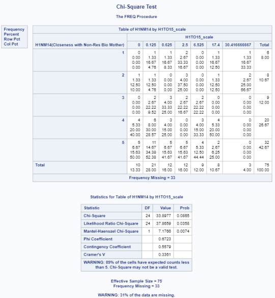
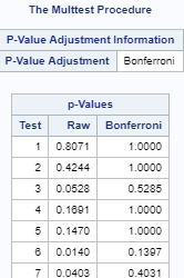
Multi-level Comparison Results

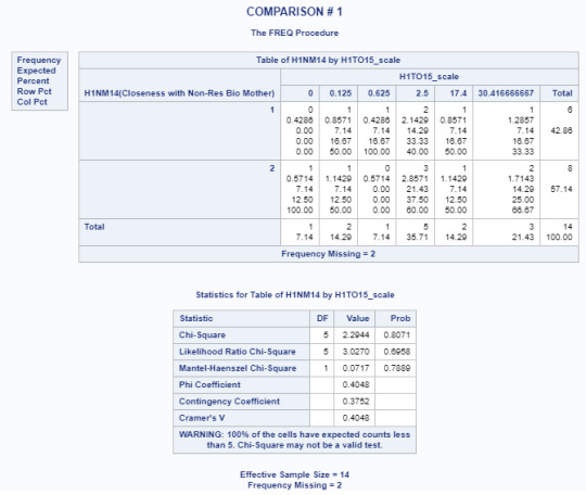
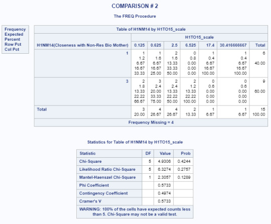
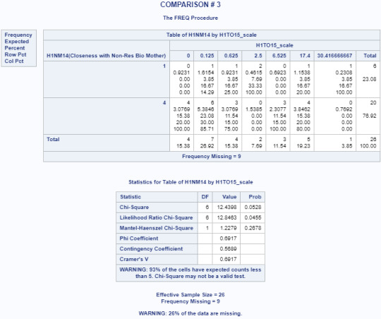
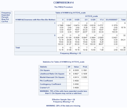
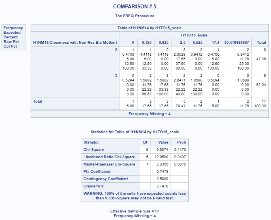
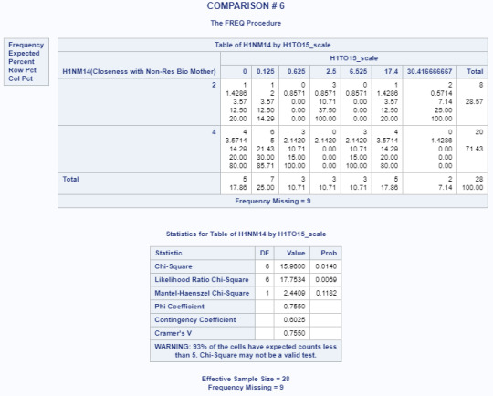
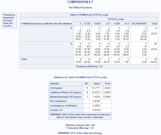
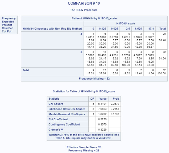
  POST HOC TEST - Bonferroni Adjustment

Had the Chi-square test of independence had a strong association (p=<0.05) between the variables, a post hoc test would have to be run in order to further provide evidence that the null hypothesis could be rejected. 

For the purposes of this exercise, given that our critical value is .05, the adjustment for the number of comparisons is closely equivalent to using a critical value of .005 (i.e., .05/10 comparisons).

Since none of these examples were lower or equal than the Bonferroni adjusted value of .05, the null hypothesis could not have been rejected for any of the post hoc tests. However, as mentioned previously, the tests would not have been run since the null hypothesis was not rejected for the initial test of main effects ”

[data-analytics-adagarzasing-blog]

Running an analysis of variance

Changes to Variables

In order to be able to work with the variables chosen for my analysis, the following changes were made:

A. Variables were collapsed in order to deal with dichotomous variables

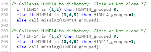
B. H1TO15="Number if Days Alcohol Consumed in Past 12 Months" was converted to reflect number of days per month and execute the analysis with a variable of the same nature as - H1TO5="Number of Days where Cigarrettes were Smoked in Past 30 Days".

ANOVA Procedure

Using ANOVA, significant differences were observed for both measures (H1TO15 & H1TO5) for both closeness to mothers and fathers. Please note that the following assumptions are made on the data and therefore it still makes sense to use this method of analysis of variance:

They were drawn from a normally distributed population

Have a common variance

Are sampled randomly and independently

Have effects that are additive.

ANOVA Results

For the purpose of this assignment, I will focus on the results based on the closeness with Mother variable as this is the main variable that showed the strongest correlation to the number of cigarettes and alcohol consumed in a period of 30 days back in the first course (Correlation procedure in previous posts). 

The ANOVA procedure, for the categorical variable H1NM14_grouped tells us that there are two levels of data (0,1). And that the analysis is based on 108 observations where adolescents had  closeness to mother scores, only 62 observations had valid scores for H1TO5. 

Upon the calculation of the one-way (ANOVA) on the number of days cigarettes were smoked in the last 30 days,  the  analysis was significant F(1, 60) = 5.09,  p = .0278. Participants found when not close to their mother, the cigarette consumption was higher (M= 24.08, SD=11.20) than when the participants were close to their mother (M= 14.7000000, SD=13.3037512).  

The ANOVA procedure, for the categorical variable H1NM14_grouped tells us that there are two levels of data (0,1). And that the analysis is based on 108 observations where adolescents had  closeness to mother scores, only 75 observations had valid scores for H1TO5. 

Upon the calculation of the one-way (ANOVA) on the number of days alcohol was consumed within the last 30 days,  the  analysis was significant F(1, 73) = 10.58, p = .0017. Participants found when not close to their mother, the cigarette consumption was higher ( M=9.96, SD=12.48) than when the participants were close to their mother (M=3.11, SD=5.26).  

POST HOC TEST

For this project, the Tukey-Kramer post hoc test has been used:

Results

Results of the post hoc test show that means between the two groups are different and therefore could support the rejection of the null hypothesis using the assumptions mentioned above.

Closeness with Mother - Grouped

The ANOVA Procedure - Tukey's Studentized Range (HSD) Test for H1TO5

Note:This test controls the Type I experimentwise error rate, but it generally has a higher Type II error rate than REGWQ.

The ANOVA Procedure - Tukey's Studentized Range (HSD) Test for H1TO15_scale

Note:This test controls the Type I experimentwise error rate, but it generally has a higher Type II error rate than REGWQ.

[data-analytics-adagarzasing-blog]

CORR Procedure

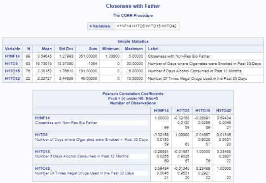
Another way to show case the information presented in this research is to use the CORR Procedure. 

Code 

The code to produce the analysis tables with all the variables earlier described in the project is presented below:

The tables that result from running the code above are shown below:

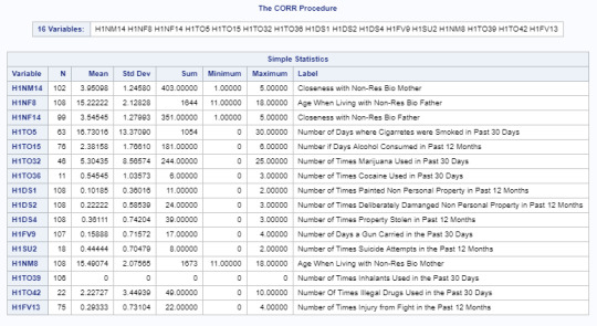
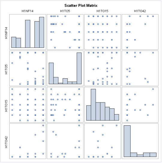
Furthermore, visual representation of this data can be added with the code below:

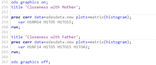
This code, produces a histogram matrix. 

I have concentrated on providing data for those variables that do in fact seem to have a correlation the perceived closeness between the adolescent towards his or her non-residential biological mother and inclination to smoke or drink.

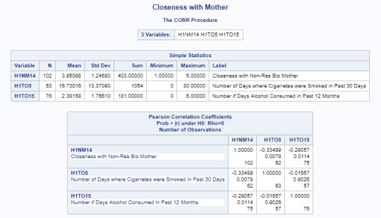
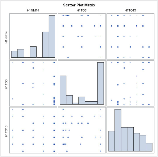
Same data is showcased below based on the perceived closeness between the adolescent towards his or her non-residential biological father and inclination to smoke, drink and use illegal drugs.

[data-analytics-adagarzasing-blog]

Assignment # 4 - Creating graphs for my data

Variables Used

For assignment # 4 and based on my research question,

Is the perceived closeness between adolescent and the non-resident parent directly correlated with risky behaviors exhibited by the adolescent?

the type of variables being dealt with are all of a categorical nature. Given that there is a categorical to categorical relationship with all my variables, this assignment will show uni-variate and bi-variate bar charts in order to visualize these relationships.

All the data management carried out for the different variables took place in assignment # 3. Please scroll down if you need to see the details.

Uni-variate Graphs

The code to create the uni-variate graphs is shown below:

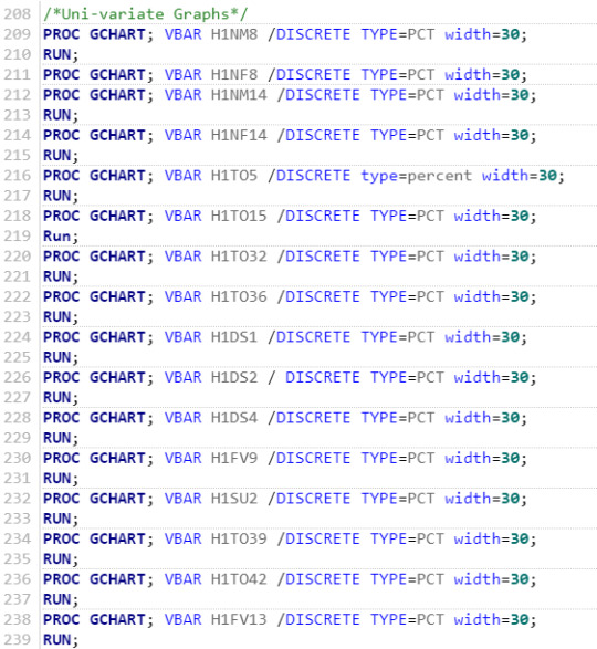
A sample of uni-variate graphs have been provided below for review. Please note this is a sample of my graphs (the most relevant ones) as there are a total of 18 variables.

H1NM8 - Age When Living with Non-Res Bio Mother

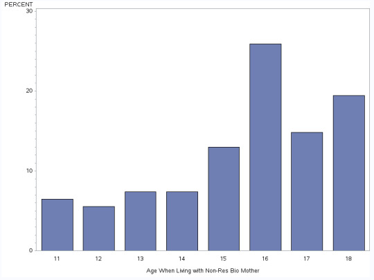
This graph is bi-modal, with a skew to the right. Its highest peak at 16 years of age and then at 18 years of age.  There is a higher frequency in the lower age ranges.

H1NF8 - Age When Living with Non-Res Bio Father

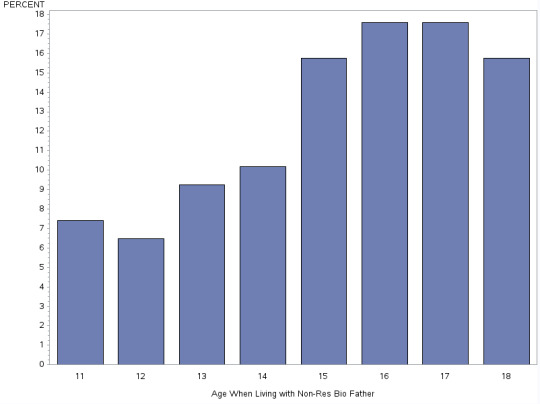
This graph is uni-modal, with a skew to the right. Its highest peak at 16 and 17 years of age. There is a higher frequency in the lower to medium age ranges.

H1NM14 - Closeness with Non-Res Bio Mother

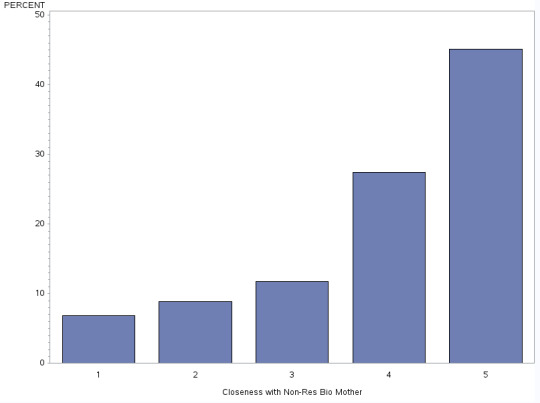
This graph is uni-modal, with a skew to the right. Its highest peak is at number 5 - which means that most of the subjects feel really close to their non resident biological mother. .

H1NF14 - Closeness with Non-Res Bio Father

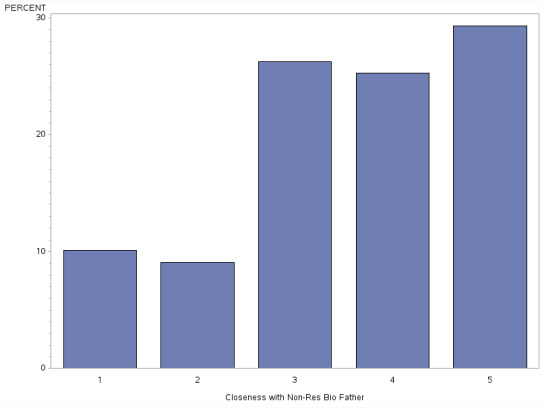
This graph uni-modal, with a skew to the right. The value of 5 is again the highest but values 3 and 4 are pretty much at par. This means that adolescents perceived to be somewhat close, quite close or extremely close to their fathers.

H1TO5 - Number of Days where Cigarettes were Smoked in Past 30 Days

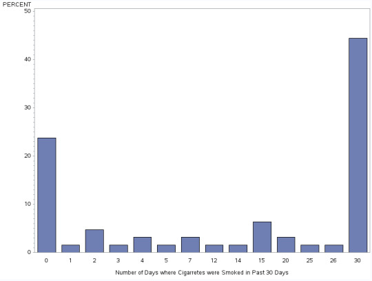
This is a bi-modal graph. The two peaks of information where about 25% of the respondents had no cigarettes (0 days) and where pretty much every day the respondents smoked cigarettes.

H1TO15 - Number of Days Alcohol Consumed in Past 12 Months

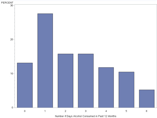
This is a uni-modal graph with a prominent skew to the left. The rest of the score are pretty similar staying at a mid to lower range.

Please note: all other variables related to risky behaviors did not provide a significant amount of data to prove correlation between perceived adolescents closeness towards non-resident biological mother or non-resident biological father. These variables were not included as part of the sample.

Bi-variate Graph

The code to create the uni-variate graphs is shown below: 

I chose to display four bi-variate graphs - between two different risky behaviors (cigarettes and alcohol consumption) and non-resident father and non-resident mother. This is due to the fact that the only data that provided significant results during my analysis to see correlation of risky behavior occurrences based on the perceived closeness of the adolescent and parent relationship.

Closeness to Non Resident Bio Mother & Cigarette Consumption

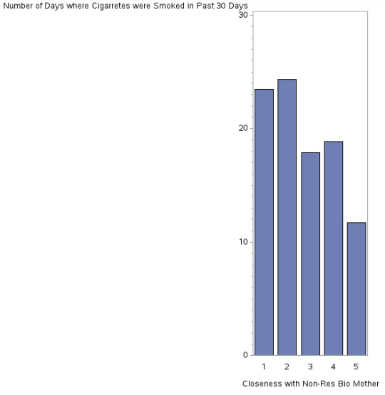
This histogram shows somewhat of a negative relationship  (as one variable increase, the other decreases) between the perceived closeness between the adolescent towards his or her non-residential biological mother and inclination to smoke. If the adolescent feels not close (x=1) or not very close (x=2) to his or her mother, the more likely they are to smoke. However, we also see high number of smoking occurrences as well when we look at the data representing that where the adolescent feels quite close to his or her mother (X=4), their chances or smoking increase. More analysis is required to determine as to why we see this pattern.

Closeness to Non Resident Bio Father & Cigarette Consumption

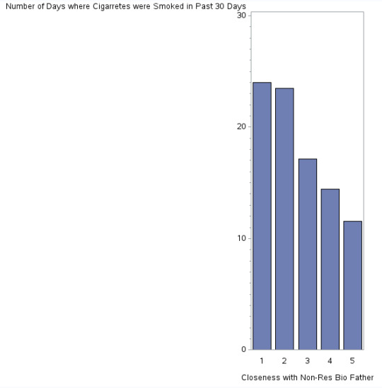
This histogram shows a negative relationship  (as one variable increase, the other decreases) between the perceived closeness between the adolescent towards his or her non-residential biological father and inclination to smoke . This means that the closer the adolescent feels towards his or her father (X axis), the least he or she will be inclined to smoke (Y axis).

Closeness to Non Resident Bio Mother & Alcohol Consumption

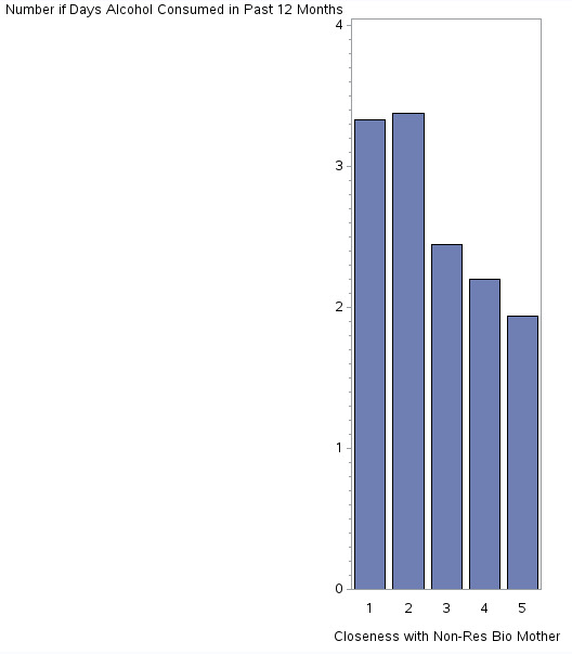
Similarly, this histogram shows a negative relationship (as one variable increase, the other decreases) between the perceived closeness between the adolescent towards his or her non-residential biological mother  and inclination to consume alcohol. This means that the closer the adolescent feels towards his or her mother (X axis), the least he or she will be inclined to consume alcohol (Y axis).

Closeness to Non Resident Bio Father & Alcohol Consumption

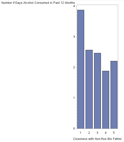
Lastly, this histogram shows somewhat of a negative relationship (as one variable increase, the other decreases) between the perceived closeness between the adolescent towards his or her non-residential biological father and inclination to consume alcohol. This means that the closer the adolescent feels towards his or her father (X axis), the least he or she will be inclined to consume alcohol (Y axis). Here, we see that for those adolescents that do not feel close to their father at all (X=1), the likelihood of them consuming alcohol is quite higher than the other responses.

[data-analytics-adagarzasing-blog]

Assignment # 3 - Making Data Management Decisions

Recap

After the initial analysis, I would like to redefine my original research question to base it only on a subset of the AddHealth data set:

Is the perceived closeness between adolescent and the non-resident parent directly correlated with risky behaviors exhibited by the adolescent?

Hypothesis

My research will demonstrate that there is is a strong correlation between the the perceived closeness between the adolescent and the non-resident parent directly correlated with risky behaviors exhibited by the adolescent

Code for Collapsing Responses 

In order to carry out my analysis there was quite a bit of data management required with my data. 

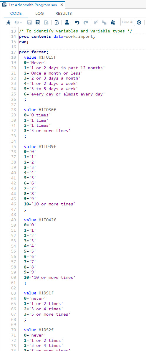
First, the responses for some of the variables where the answers had a big range of values were collapsed into more manageable rows/answers. A lot of the variables that provide insights into the different risky behaviors had up to 30 possible responses. Collapsing the responses would allow for obtaining more meaningful data.

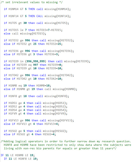
Please see sample of some of the variables and the code used to collapse responses:

Code for eliminating irrelevant responses

Another step taken for data management was to eliminate irrelevant responses to the research - that is, responses that did not provide any insights to answer my research questions and hypothesis. For this exercise, responses where the answer was not applicable (N/A),  the subject refused to answer the question (refused), the subject did not know the answer to the question (don’t know), were removed from the analysis. 

Frequency Distribution Tables

Frequency distribution tables are shown below:

/*Procedure to run the frequency distribution for all variables*/ PROC FREQ DATA=ADASDATA.NEW; TABLES H1NM8 H1NM14 H1NF8 H1NF14 H1TO5 H1TO15 H1TO32 H1TO36 H1TO39 H1TO42 H1DS1 H1DS2 H1DS4 H1FV9 H1FV13 H1SU2; /*Running the program*/ RUN;

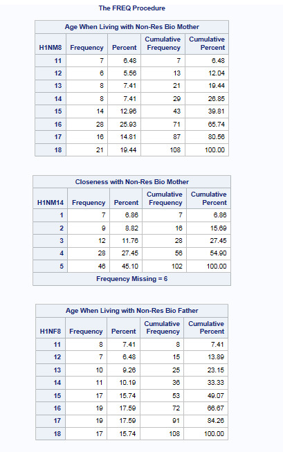
For variable H1NM8, the most endorsed answer was 16 (25.69%), where a little over 25% of the subjects lived with their non-resident biological mother at the age of 16 years of age.

For variable HQNM14, the most endorsed answer was 5 (45.10%), where over 45% of the subjects feel really close to their Non-Resident Biological Mother. Additionally, for this variable we see that there are 6 instances where responses are missing. Therefore these have been removed from the analysis and the instances are identified in the frequency tables. 

For variable H1NF8, the most endorsed answers were 16 (17.59%) and 17 (17.59%), where in both instances over 17% of the subjects lived with their non-resident biological father at the ages of 16 and 17 years of age. 

[data-analytics-adagarzasing-blog]

Assignment # 2 - Running Your First Program

Recap

The purpose of this program is to analyze AddHealth data in order to refine the research question and hypothesis below:

“Is there correlation between resident parents (mothers and fathers) and the different types of risky behaviors exhibited by some adolescents?”

“Risky behaviors (alcohol consumption, fighting and violence, tobacco usage, drug usage and suicide) in adolescence has no correlation to having a nonresident parent.”

AddHealth Code

Below is the full code worked on so far with description tags added to each set of code in order to describe its purpose:

/*Opening up the library with the data set for AddHealth*/ LIBNAME mydata "/courses/d1406ae5ba27fe300 " access=readonly;

/*Loading the dataset created based on my research*/ DATA new; set mydata.addhealth_pds;

/*Code to rename the variables that will be used as part of my research*/ LABEL H1NM7="Ever Lived with Non-Res Bio Mother" H1NM8="Age When Living with Bio Mother" H1NM14="Closeness with NonRes Bio Mother" H1NF7="Ever Lived with Bio Father" H1NF8="Age When Living with Bio Father" H1NF14="Closeness with NonRes Bio Father" H1TO5="Number of Days where Cigarrets were Smoked in Past 30 Days" H1TO15="Number if Days Alcohol Consumed in Past 12 Months" H1TO32="Number of Times Marijuana Used in Past 30 Days" H1TO36="Number of Times Cocaine Used in Past 30 Days" H1TO39="Number of Times Inhalants Used in the Past 30 Days" H1TO42="Number Of Times Illegal Drugs Used in the Past 30 Days" H1DS1="Number of Times Painted Non Personal Property in Past 12 Months" H1DS2="Number of Times Deliberately Damanged Non Personal Property in Past 12 Months" H1DS4="Number of Times Property Stolen in Past 12 Months" H1FV9="Number of Days a Gun Carried in the Past 30 Days" H1FV13="Number of Times Injury from Fight in the Past 12 Months" H1SU2="Number of Times Suicide Attempts in the Past 12 Months";

/*Adding logical operators in order to further narrow down my research question. H1NF8 and H1NM8 have been restricted to only show data where the subjects were living with bio parents for equals or greater than 11 years*/ IF H1NM8 GE 11; IF H1NF8 GE 11;

/*Procedure to sort the data by AID*/ PROC SORT; by AID;

/*Procedure to run the frequency distribution for all variables*/ PROC FREQ; TABLES H1NM7 H1NM8 H1NM14 H1NF7 H1NF8 H1NF14 H1TO5 H1TO15 H1TO32 H1TO36 H1TO39 H1TO42 H1DS1 H1DS2 H1DS4 H1FV9 H1FV13 H1SU2; /*Running the program*/ RUN;

The screenshot below demonstrate the program run in SAS:

Frequency Distribution Tables Explained

Based on the code showcased above, this section provided details on the first three variables with their respective frequency distribution.

1) Ever Lived With Bio Mother Table

In order to understand the association between resident and non resident parents and any possible impact to the adolescent’s behavior, I need to determine how many of the subjects have lived with their biological mother and how many have not lived with their biological mother.

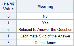
These observations can be derived by looking at the H1NM7 variable, which holds the following values:

According to the table above, 38 subjects have never lived with their biological mother. This can be seen in the H1NM7 = 0. Furthermore, this frequency also means that .7 % of the population in the data set provided this response. Conversely, H1NM7 = 1 shows that 418 subject have lived with their mother which translates to 7.95 % of the population.

For further definition on all the possible values for H1NM7 and respective frequencies, please see table below:

2) Age When Living with Bio Mother

This variable provides data on the age in which the subject was living with his/her biological mother. Since my interest is to focus on the effect of resident and non resident parents during the adolescent years, I have refined my analysis by only looking at those ages that fall under the adolescence range (11 to 19 years of age).

Each value shown in the table above for variable H1NM8 represents the age between 11 and 19 years of age.

Value 97 = Legitimate skip Value 98 = Don’t know

3) Number of Years Living with Bio Mother

This table represents the number of years the adolescent lived with his/her biological mother. The values for variable H1NM9 varies from 0 years to 19 years.

As seen in the table, 8 subjects have lived 0 years with their mother, which represents .15% of the population in he data set.

97% of the population skipped this question.This can be see when H1NM9 = 97. This begs the question as to whether this variable will give me the results I am looking for.

Research Question Redefined

After the initial analysis, I would like to redefine my original research question to base it only on a subset of the AddHealth data set:

“ Is the perceived closeness between adolescent and the non-resident parent directly correlated with risky behaviors exhibited by the adolescent?”

[data-analytics-adagarzasing-blog]

Assignment # 1 - Getting Your Research Project Started

Data Set Chosen

After taking a good look at the different code books available for this course, the one that caught my attention is the AddHealth study. 

As indicated in the course code book description, AddHealth is a representative school-based survey of adolescents in grades 7-12 in the United States. The Wave 1 survey focuses on factors that may influence adolescents’ health and risk behaviors, including personal traits, families, friendships, romantic relationships, peer groups, schools, neighborhoods, and communities.

Topics of Interest

The amount of data available in the code book is quite extensive and contains the appropriate data to explore my topic of interest: risky behaviors in adolescents in the United States.

During adolescence, some teenagers start experimenting with risky behaviors such as smoking, drinking, drugs or violence in general. Likewise, there are other teenagers that do not engage in these types of risky behaviors. This study will explore the following research question:

“Is there correlation between resident parents (mothers and fathers) and the different types of risky behaviors exhibited by some adolescents?”

Literature Used for Formulation of Hypothesis 

In order to establish a hypothesis, the following articles and journals were reviewed:

1.    Booth, Alan & Scott, Mindy & King, Valarie. (2010). Father Residence and Adolescent Problem Behavior: Are Youth Always Better Off in Two-Parent Families?. Journal of family issues. 31. 585-605. 10.1177/0192513X09351507.

Abstract

This study uses data from the National Longitudinal Study of Adolescent Health to examine combinations of father residence and closeness which have received minimal examination but involve significant numbers of children. Our findings lead to a number of conclusions. First, adolescents who are close to their nonresident fathers report higher self-esteem, less delinquency, and fewer depressive symptoms than adolescents who live with a father with whom they are not close. Second, adolescents living with a father with whom they are not close have better grades, less violence and less substance use than those having a nonresident father who is not close. At the same time, however, not being close to a resident father is associated with lower self-esteem compared to having a nonresident father who is not close. Third, adolescents do best of all when they have close ties to resident fathers. A central conclusion of this study is that it is important to consider the quality of father-child relations among those who have a resident father when assessing the impact of nonresident fathers on their children.

2.    Hetherington, E. M. (1993). An overview of the Virginia Longitudinal Study of Divorce and Remarriage with a focus on early adolescence. Journal of Family Psychology, 7(1), 39-56. http://dx.doi.org/10.1037/0893-3200.7.1.39

 Abstract

A brief summary of selected results from the Virginia Longitudinal Study of Divorce and Remarriage was presented, with a focus on findings when the children were in their early adolescent years. The early adolescent years are of particular interest in the study of the effects of parents' marital transitions on children because, at this time, problems in adjustment may emerge or intensify in children in divorced or remarried families. Furthermore, early adolescence is a time in which there is likely to be the greatest difficulty in adaptation to a new remarriage. A developmental contextual model was used to examine some of the risk, vulnerability, and protective factors associated with diverse patterns of coping with divorce and remarriage. (PsycINFO Database Record (c) 2016 APA, all rights reserved)

 3.    Manning, Wendy D., AU  - Lamb, Kathleen A., Adolescent Well-Being in Cohabiting, Married, and Single-Parent Families ,  Journal of Marriage and Family, VL  - 65, IS - 4, Blackwell Publishing Ltd, SN - 1741-3737. UR  - http://dx.doi.org/10.1111/j.1741-3737.2003.00876.x

Abstract

Cohabitation is a family form that increasingly includes children. We use the National Longitudinal Study of Adolescent Health to assess the well-being of adolescents in cohabiting parent step-families (N= 13,231). Teens living with cohabiting stepparents often fare worse than teens living with two biological married parents. Adolescents living in cohabiting step-families experience greater disadvantage than teens living in married step-families. Most of these differences, however, are explained by socioeconomic circumstances. Teenagers living with single unmarried mothers are similar to teens living with cohabiting stepparents; exceptions include greater delinquency and lower grade point averages experienced by teens living with cohabiting stepparents. Yet mother's marital history explains these differences. Our results contribute to our understanding of cohabitation and debates about the importance of marriage for children.

4.    Borawski, Elaine A., Ievers-Landis, Carolyn E., Lovegreen, Loren D., Trapl, Erika S.; Parental monitoring, negotiated unsupervised time, and parental trust: the role of perceived parenting practices in adolescent health risk behaviors,  Journal of Adolescent Health, VL  - 33, IS - 2, SP  - 60, EP  - 70, 2003/08/01/., SN  - 1054-139X. http://www.sciencedirect.com/science/article/pii/S1054139X03001009

Abstract

To compare two different parenting practices (parental monitoring and negotiated unsupervised time) and perceived parental trust in the reporting of health risk behaviors among adolescents. Data were derived from 692 adolescents in 9th and 10th grades (x̄ = 15.7 years) enrolled in health education classes in six urban high schools. Students completed a self-administered paper-based survey that assessed adolescents’ perceptions of the degree to which their parents monitor their whereabouts, are permitted to negotiate unsupervised time with their friends and trust them to make decisions. Using gender-specific multivariate logistic regression analyses, we examined the relative importance of parental monitoring, negotiated unsupervised time with peers, and parental trust in predicting reported sexual activity, sex-related protective actions (e.g., condom use, carrying protection) and substance use (alcohol, tobacco, and marijuana). For males and females, increased negotiated unsupervised time was strongly associated with increased risk behavior (e.g., sexual activity, alcohol and marijuana use) but also sex-related protective actions. In males, high parental monitoring was associated with less alcohol use and consistent condom use. Parental monitoring had no affect on female behavior. Perceived parental trust served as a protective factor against sexual activity, tobacco, and marijuana use in females, and alcohol use in males. Although monitoring is an important practice for parents of older adolescents, managing their behavior through negotiation of unsupervised time may have mixed results leading to increased experimentation with sexuality and substances, but perhaps in a more responsible way. Trust established between an adolescent female and her parents continues to be a strong deterrent for risky behaviors but appears to have little effect on behaviors of adolescent males.

5.    Kathleen Mullan Harris, Greg J. Duncan, Johanne Boisjoly; Evaluating the Role of “Nothing to Lose” Attitudes on Risky Behavior in Adolescence, Social Forces, Volume 80, Issue 3, 1 March 2002, Pages 1005–1039, https://doi.org/10.1353/sof.2002.0008

 Abstract 

This article examines the extent to which adolescents' expectations about their future in terms of health and education affect their risk-taking behavior. With data from the National Longitudinal Study of Adolescent Healthy we test the theory that a “nothing to lose” attitude about the future predicts greater involvement in risky behaviors involving early sexual intercourse, selling drugs, and weapon use. We examine the effects of both individual- and school-level conditions. Results provide mixed support for our “nothing to lose” hypothesis. We do find noteworthy school-level effects of “school climate,” including aggregate expectations, mental health, and the prevalence of single-mother families, that influence adolescent risk-taking behavior more than school measures of SES.

 6.    Elizabeth C.HairPh.D.a., M. JaneParkM.P.H.,  Thomson J.LingM.A., Kristin A.MoorePh.D.; Risky Behaviors in Late Adolescence: Co-occurrence, Predictors, and Consequences, VL  - 45, IS  - 3, SP - 253, EP  - 261, 2009/09/01/, SN  - 1054-139X, http://dx.doi.org/10.1016/j.jadohealth.2009.02.009

Abstract

Advances in research have broadened our understanding of the risky behaviors that significantly threaten adolescent health and well-being. Advances include: using person-centered, rather than behavior-centered approaches to examine how behaviors co-occur; greater focus on how environmental factors, such as family, or peer-level characteristics, influence behavior; and examination of how behaviors affect well-being in young adulthood. Use of nationally representative, longitudinal data would expand research on these critical relationships. Using data from the National Longitudinal Survey of Youth, 1997 cohort, a nationally representative sample of adolescents who are being followed over time, the present study: (1) identifies profiles of risky behaviors, (2) investigates how environmental characteristics predict these profiles of risky behaviors (e.g., delinquency, smoking, drug use, drinking, sexual behavior, and exercise), and (3) examines how these profiles of risky behaviors relate to positive and negative youth outcomes. Four “risk profiles” were identified: a high-risk group (those who report high levels of participation in numerous behaviors), a low-risk group (those who engage in very few risky behaviors), and two moderate risk-taking groups. We found that profiles with any negative behaviors were predictive of negative outcomes. It is important for practitioners to examine health behaviors in multiple domains concurrently rather than individually in isolation. Interventions and research should not simply target adolescents engaging in high levels of risky behavior but also adolescents who are engaging in lower levels of risky behaviors.

Hypothesis

After researching literature on adolescence and the effects of resident and nonresident parents, this study will try to prove the following hypothesis:

“Risky behaviors (alcohol consumption, fighting and violence, tobacco usage, drug usage and suicide) in adolescence has no correlation to having a nonresident parent.”

Personal Code Book

In order to prove my hypothesis, my personal code book will include variables on the following topics extracted from the AddHealth code book:

Section 12: Non-Resident Biological Mother

Section 13: Non-Resident Biological Father

Section 14: Resident Mother

Section 15: Resident Father

Section 16: Relations with Parents

Section 28: Tobacco, Alcohol, Drugs

Section 29: Delinquency Scale

Section 30: Joint Occurrences

Section 31: Fighting and Violence

Section 33: Suicide

Please note: the number of variables included in the code book is quite large. Therefore, only the topics of the variables relevant to the research have been included in this post.