courseraassignment

[courseraassignment]

k-Means Cluster Analysis

Week 4

Task

This week’s assignment involves running a k-means cluster analysis. Cluster analysis is an unsupervised machine learning method that partitions the observations in a data set into a smaller set of clusters where each observation belongs to only one cluster. The goal of cluster analysis is to group, or cluster, observations into subsets based on their similarity of responses on multiple variables. Clustering variables should be primarily quantitative variables, but binary variables may also be included.

this assignment is to run a k-means cluster analysis to identify subgroups of observations in your data set that have similar patterns of response on a set of clustering variables

Data

This is perhaps the best known database to be found in the pattern recognition literature. Fisher’s paper is a classic in the field and is referenced frequently to this day. (See Duda & Hart, for example.) The data set contains 3 classes of 50 instances each, where each class refers to a type of iris plant. One class is linearly separable from the other 2; the latter are NOT linearly separable from each other. Predicted attribute: class of iris plant.

Attribute Information:

sepal length in cm sepal width in cm petal length in cm petal width in cm class:Iris Setosa Iris Versicolour Iris Virginica

Results

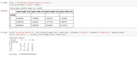
A k-means cluster analysis was conducted to identify classes of iris plants based on their similarity of responses on 4 variables that represent characteristics of the each plant bud. Clustering variables included 4 quantitative variables such as: sepal length, sepal width, petal length, and petal width. Data were randomly split into a training set that included 70% of the observations and a test set that included 30% of the observations. Then k-means cluster analyses was conducted on the training data specifying k=3 clusters (representing three classes: Iris Setosa, Iris Versicolour, Iris Virginica), using Euclidean distance. To describe the performance of a classifier and see what types of errors our classifier is making a confusion matrix was created. The accuracy score is 0.82, which is quite good due to the small number of observation (n=150).

Source Code 

import numpy as np

import pandas as pd

import matplotlib.pylab as plt

from sklearn.model_selection import train_test_split

from sklearn import datasets

from sklearn.cluster import KMeans

from sklearn.metrics import accuracy_score

from sklearn.decomposition import PCA

import seaborn as sns

%matplotlib inline

rnd_state = 3927

iris = datasets.load_iris()

data = pd.DataFrame(data= np.c_[iris[‘data’], iris[‘target’]],

columns= iris['feature_names’] + ['target’])

data.head()

data.info()

data.describe()

pca_transformed = PCA(n_components=2).fit_transform(data.iloc[:, :4])

colors=[“#9b59b6”, “#e74c3c”, “#2ecc71”]

plt.figure(figsize=(12,5))

plt.subplot(121)

plt.scatter(list(map(lambda tup: tup[0], pca_transformed)),

list(map(lambda tup: tup[1], pca_transformed)),

c=list(map(lambda col: “#9b59b6” if col==0 else “#e74c3c” if col==1 else “#2ecc71”, data.target)))

plt.title('PCA on Iris data’)

plt.subplot(122)

sns.countplot(data.target, palette=sns.color_palette(colors))

plt.title('Countplot Iris classes’);

(predictors_train, predictors_test,

target_train, target_test) = train_test_split(data.iloc[:, :4], data.target, test_size = .3, random_state = rnd_state)

classifier = KMeans(n_clusters=3).fit(predictors_train)

prediction = classifier.predict(predictors_test)

pca_transformed = PCA(n_components=2).fit_transform(predictors_test)

Predicted classes 1 and 2 mismatch the real ones, so the code block below fixes that problem.

prediction = np.where(prediction==1, 3, prediction)

prediction = np.where(prediction==2, 1, prediction)

prediction = np.where(prediction==3, 2, prediction)

plt.figure(figsize=(12,5))

plt.subplot(121)

plt.scatter(list(map(lambda tup: tup[0], pca_transformed)),

list(map(lambda tup: tup[1], pca_transformed)),

c=list(map(lambda col: “#9b59b6” if col==0 else “#e74c3c” if col==1 else “#2ecc71”, target_test)))

plt.title('PCA on Iris data, real classes’);

plt.subplot(122)

plt.scatter(list(map(lambda tup: tup[0], pca_transformed)),

list(map(lambda tup: tup[1], pca_transformed)),

c=list(map(lambda col: “#9b59b6” if col==0 else “#e74c3c” if col==1 else “#2ecc71”, prediction)))

plt.title('PCA on Iris data, predicted classes’);

clust_df = predictors_train.reset_index(level=[0])

clust_df = predictors_train.reset_index(level=[0])

clust_df.drop('index’, axis=1, inplace=True)

clust_df['cluster’] = classifier.labels_

clust_df.head()

print ('Clustering variable means by cluster’)

clust_df.groupby('cluster’).mean()

print('Confusion matrix:\n’, pd.crosstab(target_test, prediction, colnames=['Actual’], rownames=['Predicted’], margins=True))

print(’\nAccuracy: ’, accuracy_score(target_test, prediction))

Output Screenshot

[courseraassignment]

Week 3 Lasso Regression

Task

This week’s assignment involves running a lasso regression analysis. Lasso regression analysis is a shrinkage and variable selection method for linear regression models. The goal of lasso regression is to obtain the subset of predictors that minimizes prediction error for a quantitative response variable. The lasso does this by imposing a constraint on the model parameters that causes regression coefficients for some variables to shrink toward zero. Variables with a regression coefficient equal to zero after the shrinkage process are excluded from the model. Variables with non-zero regression coefficients variables are most strongly associated with the response variable. Explanatory variables can be either quantitative, categorical or both.

This assignment is to run a lasso regression analysis using k-fold cross validation to identify a subset of predictors from a larger pool of predictor variables that best predicts a quantitative response variable.

Data

Dataset description: hourly rental data spanning two years.

Dataset can be found at Kaggle

Features:

yr - year

mnth - month

season - 1 = spring, 2 = summer, 3 = fall, 4 = winter

holiday - whether the day is considered a holiday

workingday - whether the day is neither a weekend nor holiday

weathersit - 1: Clear, Few clouds, Partly cloudy, Partly cloudy

temp - temperature in Celsius

atemp - "feels like" temperature in Celsius

hum - relative humidity

windspeed (mph) - wind speed, miles per hour

windspeed (ms) - wind speed, metre per second

2: Mist + Cloudy, Mist + Broken clouds, Mist + Few clouds, Mist

3: Light Snow, Light Rain + Thunderstorm + Scattered clouds, Light Rain + Scattered clouds

4: Heavy Rain + Ice Pallets + Thunderstorm + Mist, Snow + Fog

Target:

cnt - number of total rentals

Results

A lasso regression analysis was conducted to predict a number of total bikes rentals from a pool of 12 categorical and quantitative predictor variables that best predicted a quantitative response variable. Categorical predictors included weather condition and a series of 2 binary categorical variables for holiday and workingday to improve interpretability of the selected model with fewer predictors. Quantitative predictor variables include year, month, temperature, humidity and wind speed.

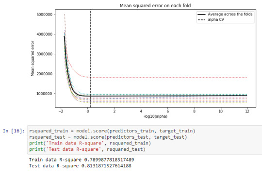
Data were randomly split into a training set that included 70% of the observations and a test set that included 30% of the observations. The least angle regression algorithm with k=10 fold cross validation was used to estimate the lasso regression model in the training set, and the model was validated using the test set. The change in the cross validation average (mean) squared error at each step was used to identify the best subset of predictor variables.

Of the 12 predictor variables, 10 were retained in the selected model:

atemp: 63.56915200306693

holiday: -282.431748735072

hum: -12.815264427009353

mnth: 0.0

season: 381.77762475080044

temp: 58.035647703871234

weathersit: -514.6381162101678

weekday: 69.84812053893549

windspeed(mph): 0.0

windspeed(ms): -95.71090321577515

workingday: 36.15135752613271

yr: 2091.5182927517903

Train data R-square 0.7899877818517489 Test data R-square 0.8131871527614188

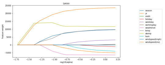
During the estimation process, year and season were most strongly associated with the number of total bikes rentals, followed by temperature and weekday. Holiday, humidity, weather condition and wind speed (ms) were negatively associated with the number of total bikes rentals.

Source code

import pandas as pd import numpy as np import matplotlib.pylab as plt from sklearn.model_selection import train_test_split from sklearn.linear_model import LassoLarsCV from sklearn import preprocessing from sklearn.metrics import mean_squared_error import seaborn as sns %matplotlib inline

rnd_state = 983

data = pd.read_csv("data/bikes_rent.csv") data.info()

data.describe()

data.head() data.dropna(inplace=True) data.iloc[:, :12].corrwith(data['cnt']) plt.figure(figsize=(15, 5)) sns.heatmap(data[['temp', 'atemp', 'hum', 'windspeed(mph)', 'windspeed(ms)', 'cnt']].corr(), annot=True, fmt='1.4f'); predictors = data.iloc[:, :12] target = data['cnt'] (predictors_train, predictors_test, target_train, target_test) = train_test_split(predictors, target, test_size = .3, random_state = rnd_state) model = LassoLarsCV(cv=10, precompute=False).fit(predictors_train, target_train) dict(zip(predictors.columns, model.coef_)) log_alphas = -np.log10(model.alphas_) plt.figure(figsize=(10, 5)) for idx, feature in enumerate(predictors.columns):    plt.plot(log_alphas, list(map(lambda r: r[idx], model.coef_path_.T)), label=feature) plt.legend(loc="upper right", bbox_to_anchor=(1.4, 0.95)) plt.xlabel("-log10(alpha)") plt.ylabel("Feature weight") plt.title("Lasso"); log_cv_alphas = -np.log10(model.cv_alphas_) plt.figure(figsize=(10, 5)) plt.plot(log_cv_alphas, model.mse_path_, ':') plt.plot(log_cv_alphas, model.mse_path_.mean(axis=-1), 'k',         label='Average across the folds', linewidth=2) plt.axvline(-np.log10(model.alpha_), linestyle='--', color='k',            label='alpha CV') plt.legend() plt.xlabel('-log10(alpha)') plt.ylabel('Mean squared error') plt.title('Mean squared error on each fold'); rsquared_train = model.score(predictors_train, target_train) rsquared_test = model.score(predictors_test, target_test) print('Train data R-square', rsquared_train) print('Test data R-square', rsquared_test)

Screen Shot of output

[courseraassignment]

Random Forest Assignment Week2

syntax codes  For Running Random Forest 

(I used adult census income dataset from kaggle.com)

from pandas import Series, DataFrame

import pandas as pd

import numpy as np

import os

import matplotlib.pylab as plt

from sklearn.model_selection import train_test_split

from sklearn.tree import DecisionTreeClassifier

from sklearn.metrics import classification_report

import sklearn.metrics

# Feature Importance

from sklearn import datasets

from sklearn.ensemble import ExtraTreesClassifier

 #Load the dataset

 AH_data = pd.read_csv('Downloads/adult.csv')

data_clean = AH_data.dropna()

data_clean.dtypes

data_clean.describe()

 #Split into training and testing sets

 predictors = data_clean[['age','fnlwgt','education.num','capital.gain','capital.loss','hours.per.week',]]

 targets = data_clean.age

 pred_train, pred_test, tar_train, tar_test  = train_test_split(predictors, targets, test_size=.4)

 pred_train.shape

pred_test.shape

tar_train.shape

tar_test.shape

 #Build model on training data

from sklearn.ensemble import RandomForestClassifier

classifier=RandomForestClassifier(n_estimators=25)

classifier=classifier.fit(pred_train,tar_train)

predictions=classifier.predict(pred_test)

sklearn.metrics.confusion_matrix(tar_test,predictions)

sklearn.metrics.accuracy_score(tar_test, predictions)

 # fit an Extra Trees model to the data

model = ExtraTreesClassifier()

model.fit(pred_train,tar_train)

# display the relative importance of each attribute

print(model.feature_importances_)

  """

Running a different number of trees and see the effect

of that on the accuracy of the prediction

"""

trees=range(25)

accuracy=np.zeros(25)

for idx in range(len(trees)):

   classifier=RandomForestClassifier(n_estimators=idx + 1)

   classifier=classifier.fit(pred_train,tar_train)

   predictions=classifier.predict(pred_test)

   accuracy[idx]=sklearn.metrics.accuracy_score(tar_test, predictions)

   plt.cla()

plt.plot(trees, accuracy)

Output Screenshot :

  Random forest analysis was performed to evaluate the importance of a series of explanatory variables in predicting a binary, categorical response variable. The following explanatory variables were included as possible contributors to a random forest The [['age','fnlwgt','education.num','capital.gain','capital.loss','hours.per.week',]]

 The variable are listed in the order [['age','fnlwgt','education.num','capital.gain','capital.loss','hours.per.week',]]

 # displaying the relative importance of each attribute

[0.81403906 0.08867596 0.02956405 0.01472304 0.00844442 0.04455346]

 And the variable with high =0.814039 and low = 0.008044059

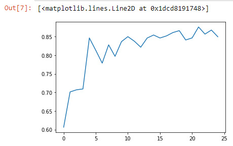
The accuracy of the random forest was 87%, with the subsequent growing of multiple trees rather than a single tree, adding little to the overall accuracy of the model, and suggesting that interpretation of a single decision tree may be appropriate.