alineonfire

[alineonfire]

COURSERA MODULE 4_WEEK 3_LASSO REGRESSION

This week, I am trying to determine what may be the reasons that influence overweight in young adults aged 10 to 20 yo, from the ADDHealth panel.

From the addhealth dataset, I manage the different variables that I need, set aside NA responses, and categorize them into binary No/Yes responses for the following topics:

TARGET VARIABLE:

H1GH28 related to weight => recoded [‘OVERWGHT’] after data management

EXPLANATORY VARIABLES (Categorical)

H1FS6 related to depression => recoded [‘DEPRESS’] after data management

H1TO15 related to alcohol habits => recoded [‘ALCOHOL’]

H1TO32 related to Majiruana consumption => recoded [‘MJCONSO’]

And I add Quantitative Explanatory Variables:

H1PF1 related to warm and love from your mother => recoded [‘LOVEMUM’] after data management

H1PF4 related to communication with your mother => recoded [‘COMMUM’]

H1PF5 related to the satisfaction of the relationship with your mother => recoded [‘RELMUM’]

The figures for each variable are therefore:

The new data set (data2) cleaned from all NA responses is now:

My sample then includes 1095 subjects.

In Python, I set predictor and target variables. Before asking for a Lasso regression, I standardize all the predictors to have a mean equal to zero and a standard deviation equal to one to get the predictors the same penalty.

As my sample includes more than 1000 subjects, I split the dataset into training data set consisting of 70% of the total observations, and the other 30% in test data set.

Once done, I run a lasso regression :

None of my predictor variables are strongly associated with overweight. Love from mother and alcohol habit have a value of zero and were subsequently removed from the model. Depressive feeling is the stronger variable associated with overweight in my selection, as well as Marijuana consumption that is negatively associated with overweight.

Let’s continue with asking for a regression coefficient progression using negativelog10 transformation to the alpha values.

Purple line is for DEPRESS, with a regression coefficient around 0.04, followed by MJCONSO (consumption of marijuana) with a negative regression coefficient -0.02. Others variables do not impact the model.

Finally, we ask Python to print the average mean square error, and test data mean square error:

The test mean square error (0.2318) is really close to the training mean square error (0.2363), meaning that both dataset have the same accuracy in predicting overweight.

The R-square values are really poor (0.02) indicating that the chosen model explained around 2% of the variance in overweight for my sample. The exercise was interesting, it still made it possible to rule out certain variables that had no impact on overweight;

[alineonfire]

COURSERA_Module 4_Week 2_Random forest

This week, I am continuing my investigations into the causes of depression in young adults aged 10 to 20 yo, from the ADDHealth panel.

From the addhealth dataset, I manage the different variables that I need, set aside NA responses, and categorize them into binary No/Yes responses for the following themes:

TARGET VARIABLE:

H1FS6: related to depression => recoded [‘DEPRESS’] after data management

EXPLANATORY VARIABLES:

H1GH28 related to weight => recoded [‘OVERWGHT’] after data management

H1TO15 related to alcohol habits => recoded [‘ALCOHOL’]

H1TO32 related to Majiruana consumption => recoded [‘MJCONSO’]

H1TO36 related to Cocaine consumption => recoded [‘COCAIN’]

The numbers for each variable are:

The new data set (data2) cleaned from NA responses is then:

My sample then includes 142 subjects on which I would like to analyse the impact of overweight, consumption of alcohol, marijuana or cocaine on depression feeling.

For this I run tree test, setting DEPRESS as target variable, and OVERWGHT, ALCOHOL, MJCONSO and COCAIN as predictors, with a size ratio to 60% for training sample and 40% for the test sample.

Predictions and confusion matrix for this test dataset are :

We can note 12  true negative, and 13 true positive responses vs 18 false negatives and 5 false positives. So only 52% of the subjects were classified correctly as depressive or not depressive.

The variable with the highest important score at 0.31 is cocaine consumption and the variable with the lowest important score is marijuana consumption at 0.15.

To refine this classification, I ask for a random forest with 25 trees, and edit the graph of accuracy values:

With my first tree, the accuracy was 52% and it seems to be a reproducible value for my dataset, as shown on the below graph. Lowest values are 48%, and highest value is 54%

Conclusion: From my point of view, the explanatory variables selected are not sufficient to correctly predict depressive feeling on young adults from my panel, other more relevant variables need to be involved.

[alineonfire]

COURSERA_MODULE 4 Week 1_ Decision tree

Before developing a decision tree, variables need to be managed. I am still working with AddHealth data set and the possible influence of an overweight and/or alcohol habit on the feeling of depression on adolescents aged 10 to 20yo.

In Python, I managed the different variables to obtain binary outcome variables :  [‘H1FS6’]: You feel depressed ? with 0=Never/rarely ; 1=sometimes ; 2=a lot of the time ; 3=Most/all of the time ; 6=Refused; 8=don’t know=> recoded as [‘DEPRESS’] with 0 (Not depressive) =0 and 1 (Depressive) including responses 1 to 3; 6 and 8 as NAN

[‘H1GH28’]: How do you think of yourself in terms of weight? and recoded it as [‘OVERWGHT’] keeping only responses 4=slightly overweight and 5=very overweight as 1 (overweight) and 3= about the right weight as 1 (Not concerned).

[‘H1TO15’]: During the past 12 months on how many days did you drink alcohol ?

with 1=everyday/almost everyday; 2= 3to5d/wk; 3= 1or2d/wk; 4= 2or3d/month; 5= 1/month or less ; 6= 1 or 2d/year ; 7= never; 96=refused; 97=legitimate skip ; 98=don’t know

=> recoded as [‘ALCOHOL’] with 0 (No alcohol habit) = 4-7 and 1 (Alcohol habits) = 1-3; 96-98 as NAN

Once done, I created a new data frame that drops all NA’S, because decision tree analysis cannot handle any NA’s in data set. This new frame is sub3clean. I set explanatory variables (OVERWGHT and ALCOHOL) and response variable (DEPRESS), and include the train test split function for predictor and target. Training sample is set as 60% and test sample is 40%.

Thus, the training sample has 1778  observations (60% of the original panel) and 2 explanatory variables, the test sample has 1186 observations and the same 2 explanatory variables. classifier.fit function give us the below results :

On the total of 1186 observations from the test sample, 460 are true negative depressive subject  (so real non-depressive people) and 206 are true positives i.e. real depressive subject.

On the other diagonal, 187 are false positives, classifying a non depressive subject as depressive, and on the other side, 333 false negative, i.e. depressive subjects classified as non-depressive.

The accuracy score is 0.56, this means that the decision tree model has classified 56% of the sample correctly as either depressive or non-depressive adolescents.

For the next step (graphic representation of the decision tree) I am very annoyed because I can’t resolve an error message that I always get in spyder :

I asked several people for help, to no avail. So frustrating !

I hope to be able to resolve this problem by the next module, in the meantime, please bear with us

Thank you

Extract from my code make a final copy of my new subsetted data

sub3=sub2.copy()

DECISION TREE

sub3clean = sub3.dropna()

sub3clean.dtypes sub3.describe()

Split into training and testing sets

predictors = sub3clean[['OVERWGHT','ALCOHOL']]

targets = sub3clean.DEPRESS

pred_train, pred_test, tar_train, tar_test = train_test_split(predictors, targets, test_size=.4)

pred_train.shape pred_test.shape tar_train.shape tar_test.shape

Build model on training data

classifier=DecisionTreeClassifier() classifier=classifier.fit(pred_train,tar_train)

predictions=classifier.predict(pred_test)

sklearn.metrics.confusion_matrix(tar_test,predictions) sklearn.metrics.accuracy_score(tar_test, predictions)

Displaying the decision tree

from sklearn import tree

from StringIO import StringIO

from io import StringIO

from StringIO import StringIO

from IPython.display import Image out = StringIO() tree.export_graphviz(classifier, out_file=out) import pydotplus graph=pydotplus.graph_from_dot_data(out.getvalue()) Image(graph.create_png())

:)

[alineonfire]

COURSERA_MODULE III _ Week 4_Logistic regression and Odds Ratios

Based on the Addhealth code,  I am interested in studying the population who declare themselves more or less depressed and the reasons which can influence this feeling. I then focused on a first phenomenon: alcohol habits.

In Python, I managed the different variables to obtain binary outcome variables (management of NAN responses, then recoding to obtain two categories 0=Not Concerned ; 1=Concerned) :   [‘H1FS6’]: You feel depressed ? with 0=Never/rarely ; 1=sometimes ; 2=a lot of the time ; 3=Most/all of the time ; 6=Refused; 8=don’t know => recoded as [‘DEPRESS’] with 0 (Not depressive) =0 and 1 (Depressive) including responses 1 to 3; 6 and 8 as NAN

[‘H1TO15’]: During the past 12 months on how many days did you drink alcohol ? with 1=everyday/almost everyday; 2= 3to5d/wk; 3= 1or2d/wk; 4= 2or3d/month; 5= 1/month or less ; 6= 1 or 2d/year ; 7= never; 96=refused; 97=legitimate skip ; 98=don’t know => recoded as [‘ALCOHOL’] with 0 (No alcohol habit) = 4-7 and 1 (Alcohol habits) = 1-3; 96-98 as NAN

Then I asked for a logistic regression and the results are :

My sample covers 3544 volunteers. P-value is 0.025, so less than 0.05. This means that alcohol habits are significantly associated with depression. Odds ratio precises that young adults (under 20yo) in this sample with alcohol habits are 1.22 times more likely to feel depressive than adults without alcohol habit.

With the standard deviations, there is 95% certainly that 2 population odds ratio fall between 1.03 and 1.45.

Nevertheless, the impact of alcohol habit on depression is quite small so let’s try to find a cofounding variable. For example the overweight.

As previously, I managed variable [‘H1GH28’]: How do you think of yourself in terms of weight? and recoded it as [‘OVERWGHT’] keeping only responses 4=slightly overweight and 5=very overweight as 1 (overweight) and 3= about the right weight as 1 (Not concerned).

The new logistic regression and odds ratios are therefore:

Number of observation is now 2964. Both alcohol habits and overweight are associated with depressive feeling as respective p-values are less than 0.05. As both variables are binary, the odds ratios can be interpreted as :

Young adults with alcohol habits are 1.35 times more likely to have depressive feeling than young adults without alcohol habit after controlling their overweight. Also overweight adults are 1.63 times more likely to feel depressive than adults with normal weight, after controlling the alcohol habits.

Because the confidence intervals on the odds ratios overlap, we can’t say that overweight is more strongly associated with depressive feeling than alcohol habits.

I used the code below on Python to have logistic regression and odds ratios :

Thank you for your reading :)

[alineonfire]

COURSERA_Module III Week 3_Multiple regression and diagnostic_My code

Below the code used for this work - graphs and results are presented in part 1 to 4 of thuis exercice. Thank you for your reading !

import pandas import numpy import seaborn import matplotlib.pyplot as plt import statsmodels.api as sm import statsmodels.formula.api as smf import statsmodels.stats.multicomp as multi import scipy.stats import scipy

bug fix for display formats to avoid run time errors

pandas.set_option('display.float_format', lambda x:'%.2f'%x)

Loading of my dataset

dataah=pandas.read_csv('addhealth_pds.csv',low_memory=False)

setting variables as numeric

dataah['H1GH51']=pandas.to_numeric(dataah['H1GH51']) dataah['H1TO15']=pandas.to_numeric(dataah['H1TO15'])

MANAGEMENT OF H1GH51: Duration of sleep

frequency distribution for each variable related to sleep habits with descriptive titles

print('Counts for H1GH51:How many hours do you usually sleep ? 96=REFUSED; 98=DONT KNOW') csl1=dataah['H1GH51'].value_counts(sort=False) print(csl1) print('Number of observations:') print(len(dataah['H1GH51']))#number of observations

management of Refused and Dont know responses as NAN for each variables

dataah['H1GH51']=dataah['H1GH51'].replace(96, numpy.nan) dataah['H1GH51']=dataah['H1GH51'].replace(98, numpy.nan) print('counts for H1GH51 with Refused, dont know responses as NAN') csl1md=dataah['H1GH51'].value_counts(sort=False, dropna=False) print(csl1md)

Descriptive statistics for quantitative variable [H1GH51]

print('describe the duration of the sleep [H1GH51]') dessl1=dataah['H1GH51'].describe() print(dessl1)

print('median') median1=dataah['H1GH51'].median() print(median1)

univariate histogram for [H1GH51] quantitative variable

dataah['H1GH51']=pandas.to_numeric(dataah['H1GH51']) seaborn.displot(dataah['H1GH51'].dropna(),kde=False) plt.xlabel('Hours of sleep') plt.title('Duration of the sleep')

Management of variable 'Marijuana consumption' H1TO32 es explanatory variable

sub1=dataah.copy() sub1['H1TO32']=pandas.to_numeric(sub1['H1TO32'])

frequency distribution for variable H1TO32 related to Consumption of Marijuana

print('Counts for H1TO32:During the past 30 days, how many times did you use marijuana? ? range 0 to 900; 996=REFUSED; 997=legitimate skip; 998=DONT KNOW; 999=Not applicable') cto1=sub1['H1TO32'].value_counts(sort=False) print(cto1) print(len(sub1['H1TO32']))#number of observations

management of Refused and non valid responses as NAN

sub1['H1TO32']=sub1['H1TO32'].replace([996,997,998,999],numpy.nan) print('counts for H1TO32 with Refused, dont know as NAN') cto2md=sub1['H1TO32'].value_counts(sort=False, dropna=False) print(cto2md)

Subset data [H1TO32] for subjects consuming = or less than 150 times/month

sub2=sub1[(sub1['H1TO32']>=0)&(sub1['H1TO32']<=150)] print('counts for subgroup H1TO32 consuming between 0 and 150 times/month') mjsub2=sub2['H1TO32'].value_counts(sort=False) print(mjsub2)

graphic representation univarie H1TO32

seaborn.distplot(sub2["H1TO32"].dropna(),kde=False) plt.xlabel('Times per month') plt.title('Consumption of marijuana')

make a copy of my new subsetted data

sub3=sub2.copy()

center Explanatory variables for regression analysis

sub3['H1TO32C']=(sub3['H1TO32']-sub3['H1TO32'].mean()) print (sub3['H1TO32C'].mean())

Regression Duration of sleep / Consomption of MJ_C

Graphic representation

Grapslmjc=seaborn.regplot(x="H1TO32C",y="H1GH51",scatter=True,data=sub3) plt.ylabel('duration of sleep') plt.xlabel('Majiruana consomption-C') plt.title('Scatterplot for the Association between Duration of sleep and Majiruana consomption-C') print(Grapslmjc)

OLS Results

slmjc=smf.ols(formula='H1GH51~H1TO32C',data=sub3).fit() print(slmjc.summary())

order=2

Grapslmjc2=seaborn.regplot(x="H1TO32C",y="H1GH51",scatter=True,order=2,data=sub3) plt.ylabel('duration of sleep_C²') plt.xlabel('Majiruana consomption') plt.title('Scatterplot for the Association between Duration of sleep and Majiruana consomption_C²') print(Grapslmjc2)

OLS Results

slmjc2=smf.ols('H1GH51~H1TO32C + I(H1TO32C**2)',data=sub3).fit() print(slmjc2.summary())

ADDITION OF ALCOHOL HABIT AS SECOND EXPLANATORY VARIABLE

Management of H1TO15: Alcohol habits

print('Counts for H1TO15: During the past 12months on how many days did you drink alcohol') print ('1=everyday/almost everyday; 2=3to5d/wk; 3=1or2d/wk; 4=2or3d/month; 5=1/month or less ; 6=1 or 2d/year ; 7=never') print('96=REFUSED; 97=legitimate skip ; 98=DONT KNOW') cal=sub3['H1TO15'].value_counts(sort=False) print(cal) print('Number of observations:') print(len(sub3['H1TO15']))#number of observations

management of Refused and Dont know responses as NAN for each variable

sub3['H1TO15']=sub3['H1TO15'].replace([96,97,98],numpy.nan) print('counts for H1TO15 with Refused, ,legitimate skip and dont know as NAN') calmd=sub3['H1TO15'].value_counts(sort=False, dropna=False) print(calmd)

make a copy of my new subsetted data

sub4=sub3.copy()

recode [H1TO15] to make sense. The more a volunteer drinks, the higher the number

recode1={1:6,2:5,3:4,4:3,5:2,6:1,7:0} sub4['ALCOHOL']=sub4['H1TO15'].map(recode1) print('counts for new variable ALCOHOL') cal2=sub4['ALCOHOL'].value_counts(sort=False, dropna=True) print(cal2)

center H1TO15 recoded as (ALCOHOL)

sub4['ALCOHOLC']=(sub4['ALCOHOL']-sub4['ALCOHOL'].mean()) print (sub4['ALCOHOLC'].mean())

suite sans H1TO632C**2 et ajout de la variable ALCOHOL centrée:

Regression Duration of sleep / Consomption of MJ_C / Consomption of alcohol

slmjcalc1=smf.ols('H1GH51~H1TO32C + ALCOHOLC' ,data=sub4).fit() print(slmjcalc1.summary())

ADEQUATION OF THE MODEL

DIAGNOSTIC #qq-plot for normality

qq1=sm.qqplot(slmjcalc1.resid, line='r')

simple plots of residuals

res1=pandas.DataFrame(slmjcalc1.resid_pearson) figr1=plt.plot(res1, 'o', ls='None') l=plt.axhline(y=0, color='r') plt.ylabel('standardized residual') plt.xlabel('Observation number') print(figr1)

additional regression diagnostic plots

figad=sm.graphics.plot_regress_exog(slmjcalc1, 'ALCOHOLC') print('figad')

leverage plot

figlev1=sm.graphics.influence_plot(slmjcalc1, size=4) print (figlev1)

[alineonfire]

COURSERA_Module III Week 3_Multiple regression and diagnostic_Part4

I perform a regression diagnostic to try to understand the cause of misspecification and ask for a qq-plot.  

The figure shows that residuals generally follow a straight line (in red) but deviate at the lower and mostly at higher quantiles. We can conclude that the residuals don’t follow perfect normal distribution.  Consumption of marijuana and alcohol arer not enough to provide an stimation of the duration of sleep. There must be other explanatory variables to consider, to improve this model.

Then, I check the graph of simple plot of residuals :

We see that the major part of the residuals falls within one standard deviation of the mean (between lines in green, -1/+1 standard deviation) or 2 standard deviation of the mean (-2/+2). However, a very large number of residues are above the absolute value of 2, which demonstrates a too high level of errors within my model. This confirms once again that the fit of my model with marijuana and alcohol consumption is poor and could be improved (with more explanatory variables)

The plot ‘Residuals versus ALCOHOC’ (in the upper right hand corner) shows the residuals for each observation at different value of alcohol consumption. There is a form of tunnel (in yellow) in which we find the absolute values of the residues in an almost symmetrical way of the axis 0. The width of the tunnel tends to decrease for the highest consumption values of alcohol.

This is consistent with other aggression diagnostic plots such as the ‘partial regression plot ‘ which indicates that this model does not predict duration of sleep for either consumers of marijuana (H1GH51), or volunteers with alcohol habits (ALCOHOLC).

Finally, we can examine the leverage of the observations:

This last graph confirms what we have already observed in the previous analysis. We have an important part of outliers, with residuals greater than 2 or less than -2 (in orange boxes), but the new information is that these outliers have small or close to zero leverage values, meaning that they do not have undue influence on the estimation of our model.  

Values in red circle have higher leverage, but they are not outliers, considering they are in the standard deviation -2/+2. There is no point which has a strong influence and which would be an outlier.

[alineonfire]

COURSERA_Module III Week 3_Multiple regression and diagnostic_ Part 3

Then I wanted to test order2 to check if this better fits the association:

Looking at OLS results, order 2 seems to be not really pertinent. Global P-value is still significant (0.002) but p-value for variable I(H1TO32C ** 2) is 0.071. We can conclude that linear regression is better than order2, the relationship between marijuana consumption and duration of sleep is rather linear than curved. So I keep linear regression in mind and try to add a second variable to refine what impacts duration of sleep. Let’s test the influence of Alcohol habit [H1TO15] (after usual management of this data with Nan, and recoding to make sense (The more a volunteer drinks, the higher the number is , then centered) :

Considering OLS results including now a panel of 1456 volunteers, new p-value is 0.00113 a little bit lower than previously. R-squared is also a little bit better but majiruana consumption and alcohol habits together, explain only 9% of the variability in duration oif sleep. We can conclude that there is clearly some error in estimating the response with this model. So, I continue with the evaluation of the adequacy of the model and the residuals (Part 4)

[alineonfire]

COURSERA Module3-WeeK3_Multiple regression and diagnostic - Part 1 and 2

In Addhealth code, I chose the variable [H1GH51] related with duration of sleep as response variable to study the influence of majiruana consumption [H1TO32] in first intention. After the usual management of both variables (distribution, NAN responses, descriptive statistics),  I kept data for marijuana consumption from 0 to 150 times/month.

Graphic representation of the association between duration of sleep and majiruana consumption , and related linear regression (with majiruana consumption centered as [H1TO32C] are : 

P-value of this analysis is 0.0029, so less than 0.005. This means that consumption of marijuana is significantly associated with duration of sleep. However, r-squared is 0.005 indicating a weak linear relationship. Not surprising, considering the data fails to adhere closely to the linear form. The  variable ‘Consumption of marijuana’ accounts only for 0.5% of the variability we see in our response variable (duration of sleep) .

The equation for the best fine line of the graph could be calculated using the ‘coef’ of the OLS regression: Duration of sleep = 7.6 – (0.0086 x consumption of marijuana)

[alineonfire]

COURSERA_Module III_Week 2_PART 3

TEST A LINEAR REGRESSION MODEL

Part 3 : Python code

Results are presented in Part 1 and Part 2 respectively, with comments. Thank you for reading :)

[alineonfire]

COURSERA_Module III_Week 2_Part 2

TEST A LINEAR REGRESSION MODEL

PART 2: Linear regression I want to investigate if the relationship between duration of sleep and sport habit is significant considering [HSleep] as explicative variable and [H1DA5] as responsive variable. First, I ask for a graphic representation as scatter plot and OLS regression:

Looking at the graph, the relation seems to be linear and positive, meaning that an increase in the duration of sleep could be associated with practicing sport more frequently.

Considering the OLS regression results:

We can conclude that the equation of the best fine line of this graph is : Duration of sleep [HSleep] = 1.38 + 0.044 [H1DA5]

The F-statistic is 20.01 and the p-value is 0.000, so really small; I can reject the null hypothesis and conclude that duration of sleep is significantly associated with sport habits.

The correlation coefficient r² is 0.003, indicates a weak linear relationship. This is not surprising considering the data fails to adhere closely to the linear form. This model accounts about 0.3% of the variability we see in our response variable, sport habits.

[alineonfire]

COURSERA_Module III_Week 2_PART 1

TEST A LINEAR REGRESSION MODEL

Part 1: Management of explicative/responsive variables

1.1: Explicative variable

I work with AddHealth code, with focus on variables [H1GH51]: ‘How many hours do you sleep ?’ as explicative variable. As previously done, I set it as numeric, ask for frequency distribution and then manage the refused or ‘don’t know’ responses as NAN.

I request descriptive statistics for this variable to have the mean, median and mode. Results are:

For the 6477 responders, the mean of duration of sleep is 7.8 (i.e 7h48min) with a standard deviation of 1.43 (+/- 1h26min). The median is 8h.

I center this original variable [H1GH51] to have a mean egal to zero (or very close to) , by subtracting the original mean value of 7.8 and check the descriptive statistics of this new variable [HSleep].

1.2 Responsive variable: I choose the variable [H1DA5] in AddHealth codebook,: ‘Did you play an active sport during past week’ as explicative variable. Responses could be : 0=not at all; 1=1 or 2 times; 2=3 or 4 times; 3=5 or more; 6=Refused; 8=Dont know' .

I run the same code as explicative variable to manage NAN response and obtain descriptive stats.

Results are:

For this variable that deals with sport habits, we have 6498 responders, the mean of sport practice  is 1.38 time/week with a standard deviation of 1.14. The median is 1time/week.

Let’s continue to investigate if the duration of sleep and the sport habits could be associated …

[alineonfire]

Coursera-Module III_Week 1/ Introduction to regression. What is your data ?

I work with the National Longitudinal Study of Adolescent Health (Addhealth Wave I) that is a merge file of three files (i) In-Home interview data (ii) parent’s questionnaire and (iii) The Add Health Picture Vocabulary Data.

Information was collected in 1994-1995, from nationally (US) representative sample of adolescents who were in grades 7-12 during the 1994-95 school year, aged 10 to 20  (Participants=6504) and their respective mother (the preferred respondent) to complete the parent questionnaire, otherwise other female head of the household, such as a legal guardian or grandmother, then father, stepfather or other male guardian.

 40 themes were addressed to the interviewer including for example daily activities, taugh in school, general health, Access to health services, feeling scale, relationship, tobacco/alcohol/drug habits, religion, … I decided to focus on Section 5 ‘Academics and Education’ gathers from all respondents, data on the progress of their schooling. Topics include absences, grades and perceptions of safety.

I note the variables

- [H1ED1]: During the 1994-1995 school year, were you absent from school for a full day with an excuse (for example, because you were sick or out of town) ? => numeric variable (int64) with range from never to more than 10 times

- [H1ED2]: During the 1994-1995 school year, how many times did you skip school for a full day without an excuse ? => object with range from 0 to 99 times (probably needed to be converted as numeric)

I also keep in mind the below variables, because I'm interested in studying the relationship with the previous ones

-  [H1ED9]: Have you ever been expelled from school ? => object, Yes/No response

- [H1ED24]: How much do you agree or disagree with the following: You feel safe in your school? => numeric variable (int64) from 1=strongly agree to 5=strongly disagree

So [H1ED1] and [H1ED2] are in my case, explanatory variables and [H1ED9] and [H1ED24] are responsive variables.

If more in-depth analysis is needed in the coming weeks, I keep aside the variable in Section 33 ‘Suicide’ collected by audio computer-assisted self interviewing (AUDIO-CASI) to test a lurking variable

-[H1SU1]: During the past 12 months, did you ever seriously think about committing suicide? => numeric variable (int64), 0=No; 1=Yes

For all the variables described: 6=refused; 7=legitimate skip and 8=don’t know, except for [H1ED2] considering 996, 997, 998 respectively and 999=not applicable.

[alineonfire]

COURSERA MODULE II_Week 4_Statistical interactions

This week deals with Statistical interactions, describing a relationship between two variables that is moderated by or dependent upon a third variable. In my example, I work with AddHealth code, and focus on variables [H1GI1Y]: year of birth and [H1DA5]: ‘Did you play an active sport during past week?’ I would like first to examine if there is a relationship between them => Does practicing an active sport impact sleep duration?

I used Python code as in the previous weeks: set variables as numeric, ask for frequency distribution, manage the ‘refused or ‘don’t know’ responses as NAN. Then, I reduce the variable H1GH51 from 1 to 10 hours of sleep and manage [H1DA5] in two sub-categories No-sport (0) and Active-Sport (1).

I ask a graphic representation of both.

Then, I perform an ANOVA test to assess the relation between both.

There are 6292 in the dataset. The p-value is very low (1.28e-12) less than 0.05 meaning that there is an association between the Sport habit and the duration of sleep. Let’s look at the means:

For people who do not practice sporting activity, the average sleep duration is 7.51 +/- 1.34 (i.e 7h31 +/- 1h20) and for people who have sport habit, the average sleep duration is 7.76 +/- 1.21 (i.e 7h46 +/- 1h13).   Now, I explore the third variable [H1TO32]: During the past 30 days, how many times did you use marijuana? Response from 0 to 900 times, 996=refused, 997 legitimate skip, 998 don’t know and 999 not applicable. I manage this variable to create a new one [MJhabit] with 2 categories No-MJ=0 for the non-consumers of marijuana and MJCONSO=1 for consumers of marijuana (response 1 to 900)

Results :

How this third variable affect the duration of sleep vs sport habits ? I explore tis question with two separate ANOVA’s:

Results

p-value is not significant (0.413) so duration of sleep vs sport habit is not impacted for people who do not consume marijuana.

In the other hand, the relationship between duration of sleep and sport habit significantly depends on consumption of marijuana.

For non consumer of marijuana, the duration of sleep is only 0.08 (5 min) different for people who practice sport or not, while the duration of sleep is longer of  0.27 (ie 16 min) for people who combine sport habit and consumption of marijuana vs people who do not practice spot, but consume marijuana.

[alineonfire]

Module II_Week 3_Pearson correlation

This week deals with Pearson Correlation, examining the association between two quantitative variables. In my example, I work with AddHealth code, with focus on variables [H1GI1Y]: year of birth and [H1GH51]: ‘How many hours do you sleep ?’ I would like to examine if there is a relationship between them.

Using Python, I check the format of these two variables => int64 and set them as numeric. I ask for the frequency distribution and them manage the refused or ‘don’t know’ responses as NAN. As both variables are Quantitative, I ask for a graphic representation as scatter plot. Looking at the graph, the relation seems to be linear and positive, meaning that an increase in the year of birth (so the younger you are) is associated with a longer duration of sleep.

However, the correlation coefficient r closed to 0.25, indicates a weak linear relationship. This is not surprising considering the data fails to adhere closely to the linear form.

r² = 0.06, meaning that we can predict only 6% of the variability we will see in the duration of sleep.

My code and results:

[alineonfire]

COURSERA _Module II week 2_ CHI TEST

I am still wondering if the duration of sleep can impact the happiness, based on the AddHealth code, with focus on variables [H1GH51]: ‘How many hours do you sleep ?’ and [H1FS11]: ‘Do you feel happy ?’

As previously done, I carried out the fundamentals which consist of studying the distribution frequencies, managing the ‘refused’ and ‘don't know’ responses as NAN, and I only kept for the variable [H1GH51] the values between 1 and 8 hours of sleep included. I controlled these steps with a graphic representation of H1GH51:

I then work on the variable [H1FS11] to recode it in two categories: ‘Not Happy’ (0) including responses 0 and 1 and ‘Happy’ (99) including responses 2 and 3 of the survey, and ask for contingency too check:

I then study the association between sleep duration and happiness using a CHI square test;

X²= 78, 9 and p-value 6E—15

X² is large and p-value very small, indicating that there is a relationship between duration of sleep and happiness. To go further, we have to perform X² test for each of the 21 possible paired comparisons. I ran this code for each of these comparison:

Results are summarized in the below table:

Adjusted p-value for 21 combination is calculated to be 0.05/21 = 0.002 based on Bonferroni adjustement.

In green, significative results for p-value < 0.002

Conclusion:

Comparisons of duration of sleep and happiness by paired, demonstrate that in fact for subjects who sleep 3, 4, 5 hours per night, the feeling of happiness is less than for subjects sleeping 7 or 8 hours per night.

If you want to feel happy in life, make sure you enough sleep :)

[alineonfire]

MODULE II_Week 1_ ANOVA test_Duration of sleep and happiness

I continue the course with my topic:  'Could the quality of sleep impact happiness?

From the AddHealth code, I focus on variables [H1GH51]: ‘How many hours do you sleep ?’ and [H1FS11]: ‘Do you feel happy ?’

Before continuing with the analysis of variance, I first went back to the fundamentals and managed my variables : Setting variables as numeric, studying the frequency distribution and managing the ‘Refused’ or ‘Don’t know’ response as NAN for both variables.

Code:

I reduce the duration of sleep from 1 to 10 hours for [H1GH51] and check the result by an univariate representation :

[H1FS11]‘Were you happy ? with  0=never or rarely; 1=sometimes; 2=a lot of the time; 3=most of the time or all of the time; 6=Refused; 8=Dont know')

Now that the data are cleaned and managed, I can proceed with analysis of variance. The response variable [H1GH51] is quantitative and the explanatory variable [H1FS11] is categorical with several level of response.

The hypothesis Ho : There is NO relationship between the happiness and duration of sleep and all means are equal ; The alternative H1 is then, There IS a relationship between the happiness and duration of sleep. 

I run the ANOVA tests on Python and ask for mean and standard deviation for [H1GH51] (hours of sleep)

And the results are :

The p-Value is 6.96E-20 << 0.05 This would allow us to reject the null hypothesis and say that the duration of sleep and happiness could be linked. But as the explanatory variable [H1FS11] has more than two levels, before concluding, I need to conduct a post hoc test, the TukeyHSD for multicomparison of the means.

And results:

This is very interesting: The ANOVA test revealed a very low p-Value, meaning that duration of sleep and happiness are significantly associated. The postHoc comparisons revealed that in fact, only subjects who responded 0-Never or rarely and 1-sometimes to the question ‘Did you feel happy’ have a different mean . The others means are statistically similar. While this, of course remains statistical, one piece of advice is that if you want to feel happy, sleep more! 😊

[alineonfire]

COURSERA WEEK4_Graphic representation

I have been continuing my research for 4 weeks now ‘How does the duration of sleep impact personality’ focusing this time on the characteristics of my variables and their graphic representations.

I reload the dataset Add Health, set variables as numeric, run a distribution of each, manage the missing data, split my main variable [H1GH51]- How many hours of sleep to you usually get-  in categories  (H1GH51 becomes sl1group4) as done and described in WEEK3.

Now I am ready for specific exercise for Week 4.

I ask Python for descriptive statistics for the H1GH51 variable, completed with median and mode parameter and graphic representation.

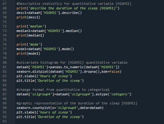
Program result is:

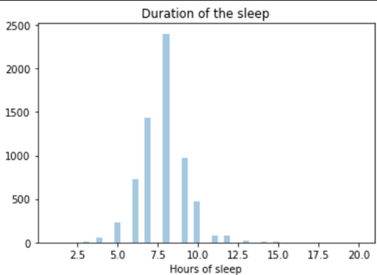
This variable is a unimodal distribution with a minimum value of 1 and maximum value of 20 hours. The mean is calculated to be 7.8 hours of sleep, close to the median equal to 8 hours.

8 is also the value with the highest frequency (mode).

I ask for representative graphic for the other variables I deal with : [H1GH52]Do you usually get enough sleep

[H1FS4] You felt that you were as good as other people

[H1SF11] You were happy

Using the code:

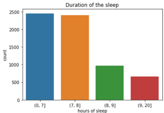
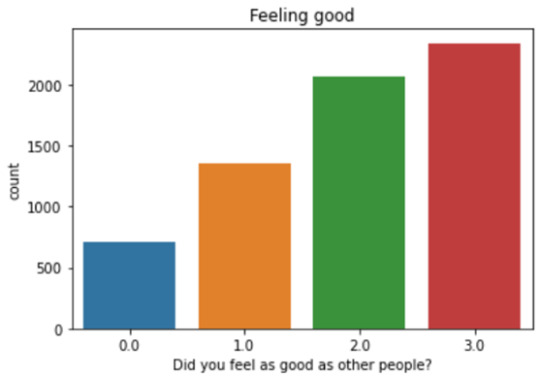
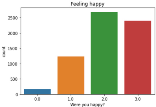
These graphs give a positive trend for the surveyed population.  It shows that a large majority of the subjects believe they had enough hours of sleep and they felt as good as other people and were happy a lot of time or all of the time. We can try to connect with the duration of sleep, to examine if the numbers of hours of sleep could impact the answer regarding the amount of sleep (enough or not) and also the feeling about self esteem and happiness

As my hypothesis is based rather on the fact that a short or very short period of sleep can influence the perception of happiness or self-esteem, I keep the variable [H1GH51] in quantitative format rather than in 4 categories. First, I ask for a bivariate graph to explore the relation between hoyurs of sleep and the perception of the duration (enough or not)

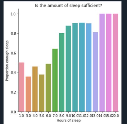
As it can be anticipated, the lower the hours of sleep, the lower the perception of having enough hours of sleep.

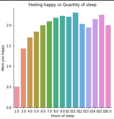
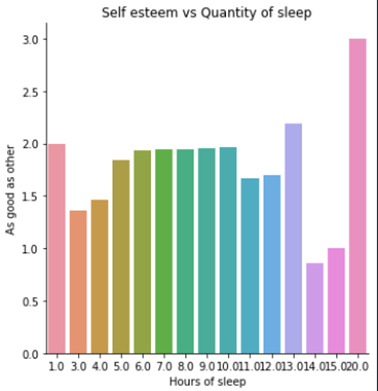
Let’s examine the impact on the perception of happiness and self-esteem :

Conclusion:

For subjects having only one hour of sleep, this seems to impact on their happiness, but not really in their self-esteem. Beyond one hour of sleep, happiness is not really impacted and keep a good level (sometimes and a lot of time, until most of the time for subjects who sleep more than 7hours).

The worst self-esteem is observed, surprisingly, in subjects who sleep a lot (14 or 15 hours by night) but becomes excellent in subjects who sleep 20 hours by night.